We’ve just announced the release of Stata 14. Stata 14 ships and downloads starting now.
Stata 14 is now available. You heard it here first.
There’s a long tradition that Statalisters hear about Stata’s new releases first. The new forum is celebrating its first birthday, but it is a continuation of the old Statalist, so the tradition continues, but updated for the modern world, where everything happens more quickly. You are hearing about Stata 14 roughly a microsecond before the rest of the world. Traditions are important.
Here’s yet another example of everything happening faster in the modern world. Rather than the announcement preceding shipping by a few weeks as in previous releases, Stata 14 ships and downloads starting now. Or rather, a microsecond from now.
Some things from the past are worth preserving, however, and one is that I get to write about the new release in my own idiosyncratic way. So let me get the marketing stuff out of the way and then I can tell you about a few things that especially interest me and might interest you.
MARKETING BEGINS.
Here’s a partial list of what’s new, a.k.a. the highlights:
- Unicode
- More than 2 billion observations (Stata/MP)
- Bayesian analysis
- IRT (Item Response Theory)
- Panel-data survival models
- Treatment effects
- Treatment effects for survival models
- Endogenous treatments
- Probability weights
- Balance analysis
- Multilevel mixed-effects survival models
- Small-sample inference for multilevel models
- SEM (structural equation modeling)
- Survival models
- Satorra-Bentler scaled chi-squared test
- Survey data
- Multilevel weights
- Power and sample size
- Survival models
- Contingency (epidemiological) tables
- Markov-switching regression models
- Tests for structural breaks in time-series
- Fractional outcome regression models
- Hurdle models
- Censored Poisson regression
- Survey support & multilevel weights for multilevel models
- New random-number generators
- Estimated marginal means and marginal effects
- Tables for multiple outcomes and levels
- Integration over unobserved and latent variables
- ICD-10
- Stata in Spanish and in Japanese
The above list is not complete; it lists about 30% of what’s new.
For all the details about Stata 14, including purchase and update information, and links to distributors outside of the US, visit stata.com/stata14.
If you are outside of the US, you can order from your authorized Stata distributor. They will supply codes so that you can access and download from stata.com.
MARKETING ENDS.
I want to write about three of the new features ‒ Unicode, more than 2-billion observations, and Bayesian analysis.
Unicode is the modern way that computers encode characters such as the letters in what you are now reading. Unicode encodes all the world’s characters, meaning I can write Hello, Здравствуйте, こんにちは, and lots more besides. Well, the forum software is modern and I always could write those words here. Now I can write them in Stata, too.
For those who care, Stata uses Unicode’s UTF-8 encoding.
Anyway, you can use Unicode characters in your data, of course; in your variable labels, of course; and in your value labels, of course. What you might not expect is that you can use Unicode in your variable names, macro names, and everywhere else Stata wants a name or identifier.
Here’s the auto data in Japanese:
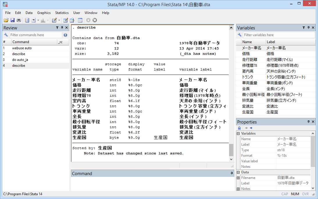
Your use of Unicode may not be as extreme as the above. It might be enough just to make tables and graphs labeled in languages other than English. If so, just set the variable labels and value labels. It doesn’t matter whether the variables are named übersetzung and kofferraum or gear_ratio and trunkspace or 変速比 and トランク.
I want to remind English speakers that Unicode includes mathematical symbols. You can use them in titles, axis labels, and the like.
Few good things come without cost. If you have been using Extended ASCII to circumvent Stata’s plain ASCII limitations, those files need to be translated to Unicode if the strings in them are to display correctly in Stata 14. This includes .dta files, do-files, ado-files, help files, and the like. It’s easier to do than you might expect. A new unicode analyze command will tell you whether you have files that need fixing and, if so, the new unicode translate command will fix them for you. It’s almost as easy as typing
. unicode translate *
This command translates your files and that has got to concern you. What if it mistranslates them? What if the power fails? Relax. unicode translate makes backups of the originals, and it keeps the backups until you delete them, which you have to do by typing
. unicode erasebackups, badidea
Yes, the option really is named badidea and it is not optional. Another unicode command can restore the backups.
The difficult part of translating your existing files is not performing the translation, it’s determining which Extended ASCII encoding your files used so that the translation can be performed. We have advice on that in the help files but, even so, some of you will only be able to narrow down the encoding to a few choices. The good news is that it is easy to try each one. You just type
. unicode retranslate *
It won’t take long to figure out which encoding works best.
Stata/MP now allows you to process datasets containing more than 2.1-billion observations. This sounds exciting, but I suspect it will interest only a few of you. How many of us have datasets with more than 2.1-billion observations? And even if you do, you will need a computer with lots of memory. This feature is useful if you have access to a 512-gigabyte, 1-terabyte, or 1.5-terabyte computer. With smaller computers, you are unlikely to have room for 2.1 billion observations. It’s exciting that such computers are available.
We increased the limit on only Stata/MP because, to exploit the higher limit, you need multiple processors. It’s easy to misjudge how much larger a 2-billion observation dataset is than a 2-million observation one. On my everyday 16 gigabyte computer ‒ which is nothing special ‒ I just fit a linear regression with six RHS variables on 2-million observations. It ran in 1.2 seconds. I used Stata/SE, and the 1.2 seconds felt fast. So, if my computer had more memory, how long would it take to fit a model on 2-billion observations? 1,200 seconds, which is to say, 20 minutes! You need Stata/MP. Stata/MP4 will reduce that to 5 minutes. Stata/MP32 will reduce that to 37.5 seconds.
By the way, if you intend to use more than 2-billion observations, be sure to click on help obs_advice that appears in the start-up notes after Stata launches. You will get better performance if you set min_memory and segmentsize to larger values. We tell you what values to set.
There’s quite a good discussion about dealing with more than 2-billion observations at stata.com/stata14/huge-datasets.
After that, it’s statistics, statistics, statistics.
Which new statistics will interest you obviously depends on your field. We’ve gone deeper into a number of fields. Treatment effects for survival models is just one example. Multilevel survival models is another. Markov-switching models is yet another. Well, you can read the list above.
Two of the new statistical features are worth mentioning, however, because they simply weren’t there previously. They are Bayesian analysis and IRT models, which are admittedly two very different things.
IRT is a highlight of the release and for some of it you will be the highlight, so I mention it, and I’ll just tell you to see stata.com/stata14/irt for more information.
Bayesian analysis is the other highlight as far as I’m concerned, and it will interest a lot of you because it cuts across fields. Many of you are already knowledgeable about this and I can just hear you asking, “Does Stata include …?” So here’s the high-speed summary:
Stata fits continuous-, binary-, ordinal-, and count-outcome models. And linear and nonlinear models. And generalized nonlinear models. Univariate, multivariate, and multiple-equation. It provides 10 likelihood models and 18 prior distributions. It also allows for user-defined likelihoods combined with built-in priors, built-in likelihoods combined with user-defined priors, and a roll-your-own programming approach to calculate the posterior density directly. MCMC methods are provided, including Adaptive Metropolis-Hastings (MH), Adaptive MH with Gibbs updates, and full Gibbs sampling for certain likelihoods and priors.
It’s also easy to use and that’s saying something.
There’s a great example of the new Bayes features in The Stata News. I mention this because including the example there is nearly a proof of ease of use. The example looks at the number of disasters in the British coal mining industry. There was a fairly abrupt decrease in the rate sometime between 1887 and 1895, which you see if you eyeballed a graph. In the example, we model the number of disasters before the change point as one Poisson process; the number after, as another Poisson process; and then we fit a model of the two Poisson parameters and the date of change. For the change point it uses a uniform prior on [1851, 1962] ‒ the range of the data ‒ and obtains a posterior mean estimate of 1890.4 and a 95% credible interval of [1886, 1896], which agrees with our visual assessment.
I hope something I’ve written above interests you. Visit stata.com/stata14 for more information.