Comparing predictions after arima with manual computations
Some of our users have asked about the way predictions are computed after fitting their models with arima. Those users report that they cannot reproduce the complete set of forecasts manually when the model contains MA terms. They specifically refer that they are not able to get the exact values for the first few predicted periods. The reason for the difference between their manual results and the forecasts obtained with predict after arima is the way the starting values and the recursive predictions are computed. While Stata uses the Kalman filter to compute the forecasts based on the state space representation of the model, users reporting differences compute their forecasts with a different estimator that is based on the recursions derived from the ARIMA representation of the model. Both estimators are consistent but they produce slightly different results for the first few forecasting periods.
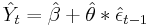
When using the postestimation command predict after fitting their MA(1) model with arima, some users claim that they should be able to reproduce the predictions with
![]()
where
![]()
However, the recursive formula for the Kalman filter prediction is based on the shrunk error (See section 13.3 in Hamilton (1993) for the complete derivation based on the state space representation):
![]()
where
![]()
![]() : is the estimated variance of the white noise disturbance
: is the estimated variance of the white noise disturbance
![]() : corresponds to the unconditional mean for the error term
: corresponds to the unconditional mean for the error term
Let’s use one of the datasets available from our website to fit a MA(1) model and compute the predictions based on the Kalman filter recursions formulated above:
** Predictions with Kalman Filter recursions (obtained with -predict- **
use http://www.stata-press.com/data/r12/lutkepohl, clear
arima dlinvestment, ma(1)
predict double yhat

** Coefficient estimates and sigma^2 from ereturn list **
scalar beta = _b[_cons]
scalar theta = [ARMA]_b[L1.ma]
scalar sigma2 = e(sigma)^2

** pt and shrinking factor for the first two observations**
generate double pt=sigma2 in 1/2
generate double sh_factor=(sigma2)/(sigma2+theta^2*pt) in 2

** Predicted series and errors for the first two observations **
generate double my_yhat = beta
generate double myehat = sh_factor*(dlinvestment - my_yhat) in 2

** Predictions with the Kalman filter recursions **
quietly {
    forvalues i = 3/91 {
        replace my_yhat = my_yhat + theta*l.myehat in `i'
        replace pt= (sigma2*theta^2*L.pt)/(sigma2+theta^2*L.pt) in `i'
        replace sh_factor=(sigma2)/(sigma2+theta^2*pt)          in `i'
        replace myehat=sh_factor*(dlinvestment - my_yhat)       in `i'
    }
}
List the first 10 predictions (yhat from predict and my_yhat from the manual computations):
. list qtr yhat my_yhat pt sh_factor in 1/10

     +--------------------------------------------------------+
     |    qtr        yhat     my_yhat          pt   sh_factor |
     |--------------------------------------------------------|
  1. | 1960q1   .01686688   .01686688   .00192542           . |
  2. | 1960q2   .01686688   .01686688   .00192542   .97272668 |
  3. | 1960q3   .02052151   .02052151   .00005251   .99923589 |
  4. | 1960q4   .01478403   .01478403   1.471e-06   .99997858 |
  5. | 1961q1   .01312365   .01312365   4.125e-08    .9999994 |
     |--------------------------------------------------------|
  6. | 1961q2   .00326376   .00326376   1.157e-09   .99999998 |
  7. | 1961q3   .02471242   .02471242   3.243e-11           1 |
  8. | 1961q4   .01691061   .01691061   9.092e-13           1 |
  9. | 1962q1   .01412974   .01412974   2.549e-14           1 |
 10. | 1962q2   .00643301   .00643301   7.147e-16           1 |
     +--------------------------------------------------------+
Notice that the shrinking factor (sh_factor) tends to 1 as t increases, which implies that after a few initial periods the predictions produced with the Kalman filter recursions become exactly the same as the ones produced by the formula at the top of this entry for the recursions derived from the ARIMA representation of the model.
Reference:
Hamilton, James. 1994. Time Series Analysis. Princeton University Press.