margins is a powerful tool to obtain predictive margins, marginal predictions, and marginal effects. It is so powerful that it can work with any functional form of our estimated parameters by using the expression() option. I am going to show you how to obtain proportional changes of an outcome with respect to changes in the covariates using two different approaches for linear and nonlinear models. Read more…

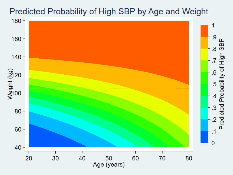
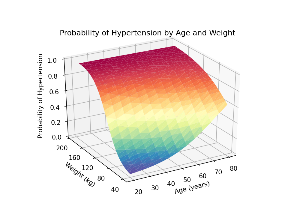
In my first four posts about Stata and Python, I showed you how to set up Stata to use Python, three ways to use Python in Stata, how to install Python packages, and how to use Python packages. It might be helpful to read those posts before you continue with this post if you are not familiar with Python. Now, I’d like to shift our focus to some practical uses of Python within Stata. This post will demonstrate how to use Stata to estimate marginal predictions from a logistic regression model and use Python to create a three-dimensional surface plot of those predictions.

Read more…

I have a confession. I wasn’t excited about the addition of frames to Stata 16. Yes, frames has been one of the most requested features for many years, and our website analytics show that frames is wildly popular. Adding frames was a smart decision and our customers are excited. But I have used Stata for over 20 years, and I have been perfectly happy using one dataset at a time. So I ignored frames.

Then I started working on an example for lasso using genetic data. I simulated patient data along with genetic data for each of 22 chromosomes saved in 22 separate datasets. Working with 23 datasets became cumbersome, so I thought I’d check out frames. I began by reading the manual and then tinkered with my genetic data. Along the way, I discovered a feature of frames that completely blew my mind. I’m going to show you that feature below, and I expect that it will blow your mind as well.

This blog post is not meant to be an introduction to frames. There is a detailed introduction to frames in the Stata 16 manual that will make you an expert. I simply want to show you some of the useful things that you can do with frames, including the following: Read more…

In his blog post, Enrique Pinzon discussed how to perform regression when we don’t want to make any assumptions about functional form—use the npregress command. He concluded by asking and answering a few questions about the results using the margins and marginsplot commands.

Recently, I have been thinking about all the different types of questions that we could answer using margins after nonparametric regression, or really after any type of regression. margins and marginsplot are powerful tools for exploring the results of a model and drawing many kinds of inferences. In this post, I will show you how to ask and answer very specific questions and how to explore the entire response surface based on the results of your nonparametric regression.
Read more…

We discuss estimating population-averaged parameters when some of the data are missing. In particular, we show how to use gmm to estimate population-averaged parameters for a probit model when the process that causes some of the data to be missing is a function of observable covariates and a random process that is independent of the outcome. This type of missing data is known as missing at random, selection on observables, and exogenous sample selection.

This is a follow-up to an earlier post where we estimated the parameters of a probit model under endogenous sample selection (http://blog.stata.com/2015/11/05/using-mlexp-to-estimate-endogenous-treatment-effects-in-a-probit-model/). In endogenous sample selection, the random process that affects which observations are missing is correlated with an unobservable random process that affects the outcome. Read more…

In Stata 14.2, we added the ability to use margins to estimate covariate effects after gmm. In this post, I illustrate how to use margins and marginsplot after gmm to estimate covariate effects for a probit model.

Margins are statistics calculated from predictions of a previously fit model at fixed values of some covariates and averaging or otherwise integrating over the remaining covariates. They can be used to estimate population average parameters like the marginal mean, average treatment effect, or the average effect of a covariate on the conditional mean. I will demonstrate how using margins is useful after estimating a model with the generalized method of moments. Read more…

I want to estimate, graph, and interpret the effects of nonlinear models with interactions of continuous and discrete variables. The results I am after are not trivial, but obtaining what I want using margins, marginsplot, and factor-variable notation is straightforward. Read more…

We continue with the series of posts where we illustrate how to obtain correct standard errors and marginal effects for models with multiple steps. In this post, we estimate the marginal effects and standard errors for a hurdle model with two hurdles and a lognormal outcome using mlexp. mlexp allows us to estimate parameters for multiequation models using maximum likelihood. In the last post (Multiple equation models: Estimation and marginal effects using gsem), we used gsem to estimate marginal effects and standard errors for a hurdle model with two hurdles and an exponential mean outcome.

We exploit the fact that the hurdle-model likelihood is separable and the joint log likelihood is the sum of the individual hurdle and outcome log likelihoods. We estimate the parameters of each hurdle and the outcome separately to get initial values. Then, we use mlexp to estimate the parameters of the model and margins to obtain marginal effects. Read more…

Starting point: A hurdle model with multiple hurdles

In a sequence of posts, we are going to illustrate how to obtain correct standard errors and marginal effects for models with multiple steps.

Our inspiration for this post is an old Statalist inquiry about how to obtain marginal effects for a hurdle model with more than one hurdle (http://www.statalist.org/forums/forum/general-stata-discussion/general/1337504-estimating-marginal-effect-for-triple-hurdle-model). Hurdle models have the appealing property that their likelihood is separable. Each hurdle has its own likelihood and regressors. You can estimate each one of these hurdles separately to obtain point estimates. However, you cannot get standard errors or marginal effects this way.

In this post, Read more…

I use features new to Stata 14.1 to estimate an average treatment effect (ATE) for a heteroskedastic probit model with an endogenous treatment. In 14.1, we added new prediction statistics after mlexp that margins can use to estimate an ATE.

I am building on a previous post in which I demonstrated how to use mlexp to estimate the parameters of a probit model with an endogenous treatment and used margins to estimate the ATE for the model Using mlexp to estimate endogenous treatment effects in a probit model. Currently, no official commands estimate the heteroskedastic probit model with an endogenous treatment, so in this post I show how mlexp can be used to extend the models estimated by Stata. Read more…