I discuss a sequence of ado-commands that use Mata to estimate the mean of a variable. The commands illustrate a general structure for Stata/Mata programs. This post builds on Programming an estimation command in Stata: Mata 101, Programming an estimation command in Stata: Mata functions, and Programming an estimation command in Stata: A first ado-command.

This is the thirteenth post in the series Programming an estimation command in Stata. I recommend that you start at the beginning. See Programming an estimation command in Stata: A map to posted entries for a map to all the posts in this series.

Using Mata in ado-programs

I begin by reviewing the structure in mymean5.ado, which I discussed Read more…

I show how to write a function in Mata, the matrix programming language that is part of Stata. This post uses concepts introduced in Programming an estimation command in Stata: Mata 101.

This is the twelfth post in the series Programming an estimation command in Stata. I recommend that you start at the beginning. See Programming an estimation command in Stata: A map to posted entries for a map to all the posts in this series.

Mata functions

Commands do work in Stata. Functions do work in Mata. Commands operate on Stata objects, like variables, and users specify options to alter the behavior. Mata functions accept arguments, operate on the arguments, and may return a result or alter the value of an argument to contain a result.

Consider myadd() defined below.

mata:
function myadd(X, Y)
{
    A = X + Y
    return(A)
}
end

myadd() accepts two arguments, X and Y, puts the sum of X and Y into A, and returns A. For example, Read more…

Converting a string date

Stata has a wide array of tools to work with dates. You can have dates in years, months, or even milliseconds. In this post, I will provide a brief tour of working with dates that will help you get started using all of Stata’s tools.

When you load a dataset, you will notice that every variable has a display format. For date variables, the display format is %td for daily dates, %tm for monthly dates, etc. Let’s load the wpi1 dataset as Read more…

Reflecting on the year, Stata has a lot to be thankful for—we released Stata 14, celebrated 30 years of Stata, and had the pleasure of meeting and working with many great people, including our Stata Press authors.

Are you interested in writing a book about Stata or just a book on statistics? We’d love to work with you too. Stata Press offers books with clear, step-by-step examples that make learning and teaching easier. Read more about our submission guidelines, or contact us to get started.

If you’re searching for a good book to read during the holidays, check out our full list of books or our most recent ones below. If you’d like to be notified when new books are released, sign up for Stata Press email alerts.

I hope you all have a great New Year!

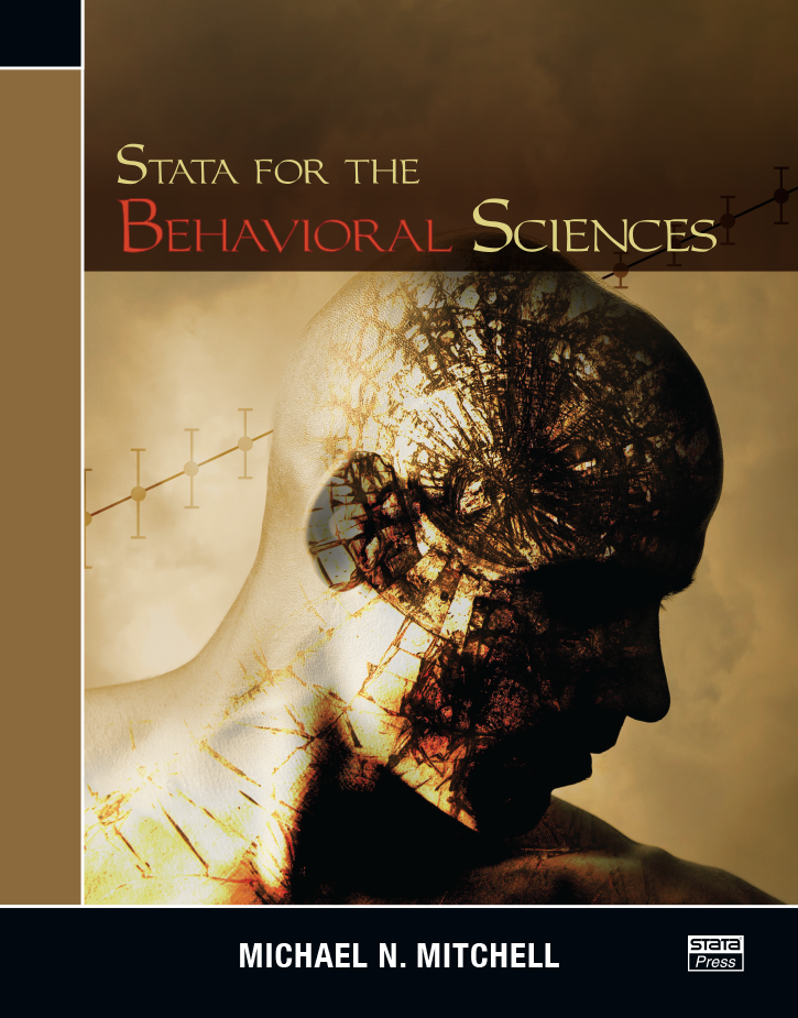
Stata for the Behavioral Sciences

Michael N. Mitchell’s Stata for the Behavioral Sciences is an ideal reference for Read more…

I introduce Mata, the matrix programming language that is part of Stata.

This is the eleventh post in the series Programming an estimation command in Stata. I recommend that you start at the beginning. See Programming an estimation command in Stata: A map to posted entries for a map to all the posts in this series. Read more…

I use features new to Stata 14.1 to estimate an average treatment effect (ATE) for a heteroskedastic probit model with an endogenous treatment. In 14.1, we added new prediction statistics after mlexp that margins can use to estimate an ATE.

I am building on a previous post in which I demonstrated how to use mlexp to estimate the parameters of a probit model with an endogenous treatment and used margins to estimate the ATE for the model Using mlexp to estimate endogenous treatment effects in a probit model. Currently, no official commands estimate the heteroskedastic probit model with an endogenous treatment, so in this post I show how mlexp can be used to extend the models estimated by Stata. Read more…

I make two improvements to the command that implements the ordinary least-squares (OLS) estimator that I discussed in Programming an estimation command in Stata: Allowing for options. First, I add an option for a cluster-robust estimator of the variance-covariance of the estimator (VCE). Second, I make the command accept the modern syntax for either a robust or a cluster-robust estimator of the VCE. In the process, I use subroutines in my ado-program to facilitate the parsing, and I discuss some advanced parsing tricks.

This is the tenth post in the series Programming an estimation command in Stata. I recommend that you start at the beginning. See Programming an estimation command in Stata: A map to posted entries for a map to all the posts in this series. Read more…

\(\newcommand{\Eb}{{\bf E}}\)This post was written jointly with Enrique Pinzon, Senior Econometrician, StataCorp.

The generalized method of moments (GMM) is a method for constructing estimators, analogous to maximum likelihood (ML). GMM uses assumptions about specific moments of the random variables instead of assumptions about the entire distribution, which makes GMM more robust than ML, at the cost of some efficiency. The assumptions are called moment conditions.

GMM generalizes the method of moments (MM) by allowing the number of moment conditions to be greater than the number of parameters. Using these extra moment conditions makes GMM more efficient than MM. When there are more moment conditions than parameters, the estimator is said to be overidentified. GMM can efficiently combine the moment conditions when the estimator is overidentified.

We illustrate these points by estimating the mean of a \(\chi^2(1)\) by MM, ML, a simple GMM estimator, and an efficient GMM estimator. This example builds on Efficiency comparisons by Monte Carlo simulation and is similar in spirit to the example in Wooldridge (2001). Read more…

I make three improvements to the command that implements the ordinary least-squares (OLS) estimator that I discussed in Programming an estimation command in Stata: Allowing for sample restrictions and factor variables. First, I allow the user to request a robust estimator of the variance-covariance of the estimator (VCE). Second, I allow the user to suppress the constant term. Third, I store the residual degrees of freedom in e(df_r) so that test will use the \(t\) or \(F\) distribution instead of the normal or \(\chi^2\) distribution to compute the \(p\)-value of Wald tests.

This is the ninth post in the series Programming an estimation command in Stata. I recommend that you start at the beginning. See Programming an estimation command in Stata: A map to posted entries for a map to all the posts in this series. Read more…

I modify the ordinary least-squares (OLS) command discussed in Programming an estimation command in Stata: A better OLS command to allow for sample restrictions, to handle missing values, to allow for factor variables, and to deal with perfectly collinear variables.

This is the eighth post in the series Programming an estimation command in Stata. I recommend that you start at the beginning. See Programming an estimation command in Stata: A map to posted entries for a map to all the posts in this series. Read more…