Multilevel linear models in Stata, part 2: Longitudinal data
In my last posting, I introduced you to the concepts of hierarchical or “multilevel” data. In today’s post, I’d like to show you how to use multilevel modeling techniques to analyse longitudinal data with Stata’s xtmixed command.
Last time, we noticed that our data had two features. First, we noticed that the means within each level of the hierarchy were different from each other and we incorporated that into our data analysis by fitting a “variance component” model using Stata’s xtmixed command.
The second feature that we noticed is that repeated measurement of GSP showed an upward trend. We’ll pick up where we left off last time and stick to the concepts again and you can refer to the references at the end to learn more about the details.
The videos
Stata has a very friendly dialog box that can assist you in building multilevel models. If you would like a brief introduction using the GUI, you can watch a demonstration on Stata’s YouTube Channel:
Introduction to multilevel linear models in Stata, part 2: Longitudinal data
Longitudinal data
I’m often asked by beginning data analysts – “What’s the difference between longitudinal data and time-series data? Aren’t they the same thing?”.
The confusion is understandable — both types of data involve some measurement of time. But the answer is no, they are not the same thing.
Univariate time series data typically arise from the collection of many data points over time from a single source, such as from a person, country, financial instrument, etc.
Longitudinal data typically arise from collecting a few observations over time from many sources, such as a few blood pressure measurements from many people.
There are some multivariate time series that blur this distinction but a rule of thumb for distinguishing between the two is that time series have more repeated observations than subjects while longitudinal data have more subjects than repeated observations.
Because our GSP data from last time involve 17 measurements from 48 states (more sources than measurements), we will treat them as longitudinal data.
GSP Data: http://www.stata-press.com/data/r12/productivity.dta
Random intercept models
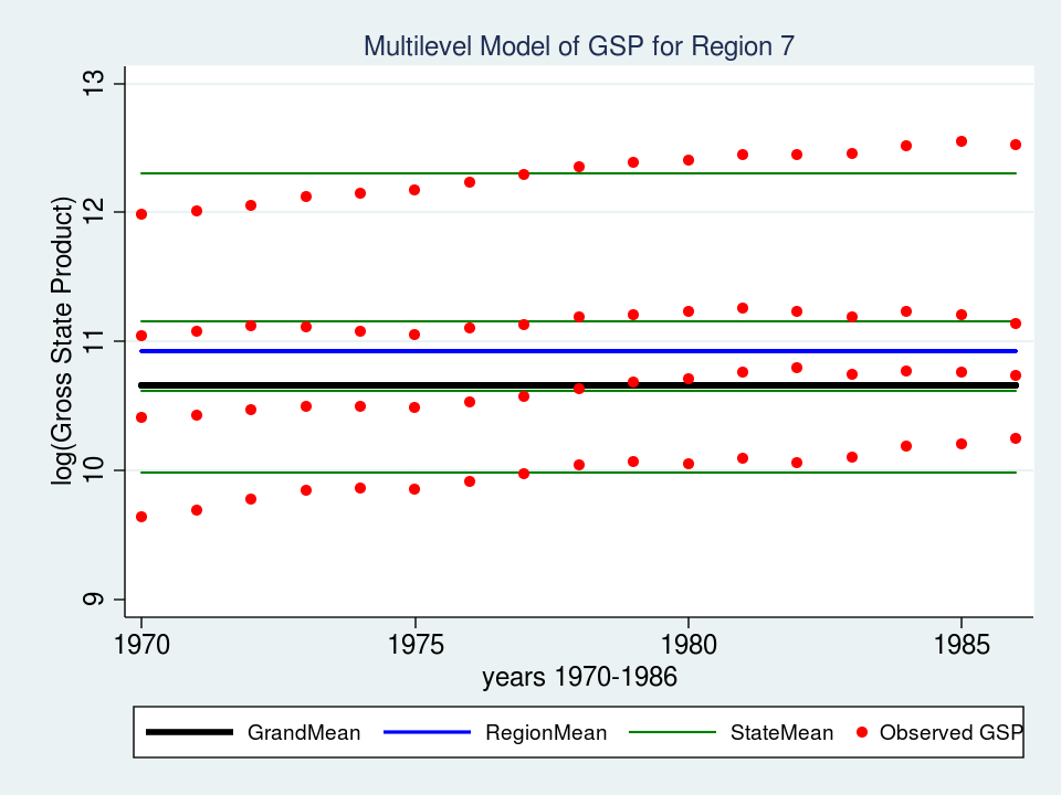
As I mentioned last time, repeated observations on a group of individuals can be conceptualized as multilevel data and modeled just as any other multilevel data. We left off last time with a variance component model for GSP (Gross State Product, logged) and noted that our model assumed a constant GSP over time while the data showed a clear upward trend.
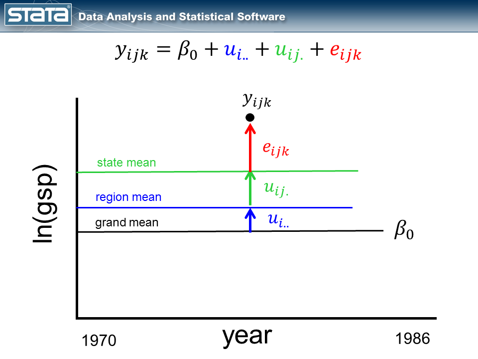
If we consider a single observation and think about our model, nothing in the fixed or random part of the models is a function of time.
Let’s begin by adding the variable year to the fixed part of our model.
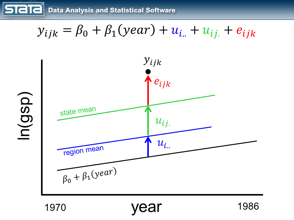
As we expected, our grand mean has become a linear regression which more accurately reflects the change over time in GSP. What might be unexpected is that each state’s and region’s mean has changed as well and now has the same slope as the regression line. This is because none of the random components of our model are a function of time. Let’s fit this model with the xtmixed command:
. xtmixed gsp year, || region: || state:

------------------------------------------------------------------------------
         gsp |      Coef.   Std. Err.      z    P>|z|     [95% Conf. Interval]
-------------+----------------------------------------------------------------
        year |   .0274903   .0005247    52.39   0.000     .0264618    .0285188
       _cons |  -43.71617   1.067718   -40.94   0.000    -45.80886   -41.62348
------------------------------------------------------------------------------

------------------------------------------------------------------------------
  Random-effects Parameters  |   Estimate   Std. Err.     [95% Conf. Interval]
-----------------------------+------------------------------------------------
region: Identity             |
                   sd(_cons) |   .6615238   .2038949      .3615664    1.210327
-----------------------------+------------------------------------------------
state: Identity              |
                   sd(_cons) |   .7805107   .0885788      .6248525    .9749452
-----------------------------+------------------------------------------------
                sd(Residual) |   .0734343   .0018737      .0698522    .0772001
------------------------------------------------------------------------------
The fixed part of our model now displays an estimate of the intercept (_cons = -43.7) and the slope (year = 0.027). Let’s graph the model for Region 7 and see if it fits the data better than the variance component model.
predict GrandMean, xb
label var GrandMean "GrandMean"
predict RegionEffect, reffects level(region)
predict StateEffect, reffects level(state)
gen RegionMean = GrandMean + RegionEffect
gen StateMean = GrandMean + RegionEffect + StateEffect

twoway  (line GrandMean year, lcolor(black) lwidth(thick))      ///
        (line RegionMean year, lcolor(blue) lwidth(medthick))   ///
        (line StateMean year, lcolor(green) connect(ascending)) ///
        (scatter gsp year, mcolor(red) msize(medsmall))         ///
        if region ==7,                                          ///
        ytitle(log(Gross State Product), margin(medsmall))      ///
        legend(cols(4) size(small))                             ///
        title("Multilevel Model of GSP for Region 7", size(medsmall))
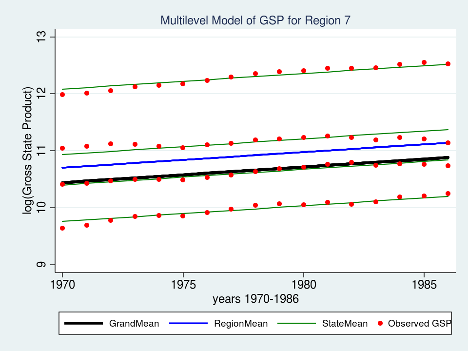
That looks like a much better fit than our variance-components model from last time. Perhaps I should leave well enough alone, but I can’t help noticing that the slopes of the green lines for each state don’t fit as well as they could. The top green line fits nicely but the second from the top looks like it slopes upward more than is necessary. That’s the best fit we can achieve if the regression lines are forced to be parallel to each other. But what if the lines were not forced to be parallel? What if we could fit a “mini-regression model” for each state within the context of my overall multilevel model. Well, good news — we can!
Random slope models
By introducing the variable year to the fixed part of the model, we turned our grand mean into a regression line. Next I’d like to incorporate the variable year into the random part of the model. By introducing a fourth random component that is a function of time, I am effectively estimating a separate regression line within each state.
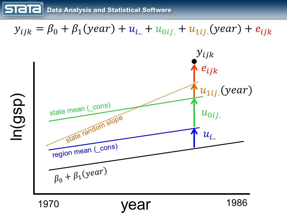
Notice that the size of the new, brown deviation u1ij. is a function of time. If the observation were one year to the left, u1ij. would be smaller and if the observation were one year to the right, u1ij.would be larger.
It is common to “center” the time variable before fitting these kinds of models. Explaining why is for another day. The quick answer is that, at some point during the fitting of the model, Stata will have to compute the equivalent of the inverse of the square of year. For the year 1986 this turns out to be 2.535e-07. That’s a fairly small number and if we multiply it by another small number…well, you get the idea. By centering age (e.g. cyear = year – 1978), we get a more reasonable number for 1986 (0.01). (Hint: If you have problems with your model converging and you have large values for time, try centering them. It won’t always help, but it might).
So let’s center our year variable by subtracting 1978 and fit a model that includes a random slope.
gen cyear = year - 1978
xtmixed gsp cyear, || region: || state: cyear, cov(indep)
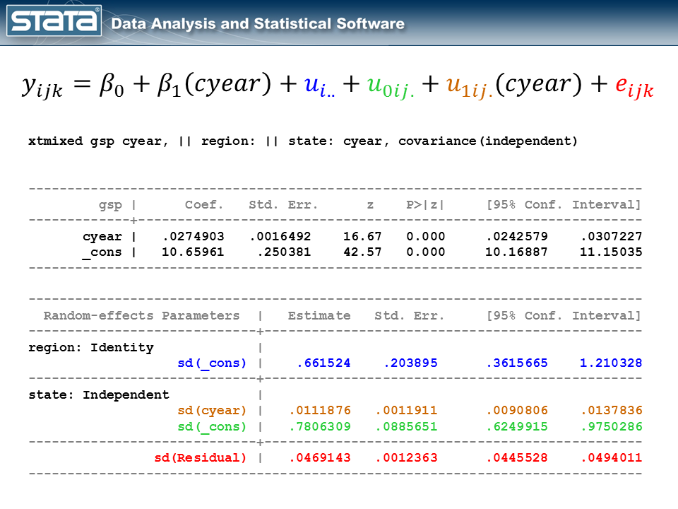
I’ve color-coded the output so that we can match each part of the output back to the model and the graph. The fixed part of the model appears in the top table and it looks like any other simple linear regression model. The random part of the model is definitely more complicated. If you get lost, look back at the graphic of the deviations and remind yourself that we have simply partitioned the deviation of each observation into four components. If we did this for every observation, the standard deviations in our output are simply the average of those deviations.
Let’s look at a graph of our new “random slope” model for Region 7 and see how well it fits our data.
predict GrandMean, xb
label var GrandMean "GrandMean"
predict RegionEffect, reffects level(region)
predict StateEffect_year StateEffect_cons, reffects level(state)

gen RegionMean = GrandMean + RegionEffect
gen StateMean_cons = GrandMean + RegionEffect + StateEffect_cons
gen StateMean_year = GrandMean + RegionEffect + StateEffect_cons + ///
                     (cyear*StateEffect_year)

twoway  (line GrandMean cyear, lcolor(black) lwidth(thick))             ///
        (line RegionMean cyear, lcolor(blue) lwidth(medthick))          ///
        (line StateMean_cons cyear, lcolor(green) connect(ascending))   ///
        (line StateMean_year cyear, lcolor(brown) connect(ascending))   ///
        (scatter gsp cyear, mcolor(red) msize(medsmall))                ///
        if region ==7,                                                  ///
        ytitle(log(Gross State Product), margin(medsmall))              ///
        legend(cols(3) size(small))                                     ///
        title("Multilevel Model of GSP for Region 7", size(medsmall))
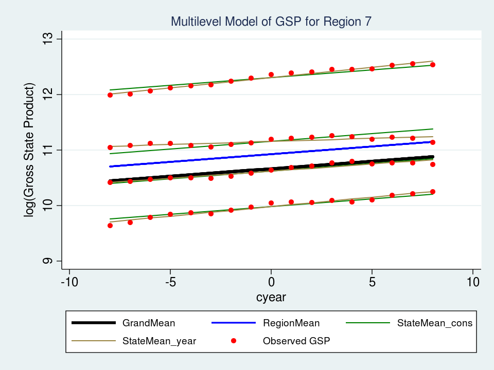
The top brown line fits the data slightly better, but the brown line below it (second from the top) is a much better fit. Mission accomplished!
Where do we go from here?
I hope I have been able to convince you that multilevel modeling is easy using Stata’s xtmixed command and that this is a tool that you will want to add to your kit. I would love to say something like “And that’s all there is to it. Go forth and build models!”, but I would be remiss if I didn’t point out that I have glossed over many critical topics.
In our GSP example, we would still like to consider the impact of other independent variables. I haven’t mentioned choice of estimation methods (ML or REML in the case of xtmixed). I’ve assessed the fit of our models by looking at graphs, an approach important but incomplete. We haven’t thought about hypothesis testing. Oh — and, all the usual residual diagnostics for linear regression such as checking for outliers, influential observations, heteroskedasticity and normality still apply….times four! But now that you understand the concepts and some of the mechanics, it shouldn’t be difficult to fill in the details. If you’d like to learn more, check out the links below.
I hope this was helpful…thanks for stopping by.
For more information
If you’d like to learn more about modeling multilevel and longitudinal data, check out
Multilevel and Longitudinal Modeling Using Stata, Third Edition
Volume I: Continuous Responses
Volume II: Categorical Responses, Counts, and Survival
by Sophia Rabe-Hesketh and Anders Skrondal
or sign up for our popular public training course Multilevel/Mixed Models Using Stata.