Unit-root tests in Stata
\(\newcommand{\mub}{{\boldsymbol{\mu}}}
\newcommand{\eb}{{\boldsymbol{e}}}
\newcommand{\betab}{\boldsymbol{\beta}}\)Determining the stationarity of a time series is a key step before embarking on any analysis. The statistical properties of most estimators in time series rely on the data being (weakly) stationary. Loosely speaking, a weakly stationary process is characterized by a time-invariant mean, variance, and autocovariance.
In most observed series, however, the presence of a trend component results in the series being nonstationary. Furthermore, the trend can be either deterministic or stochastic, depending on which appropriate transformations must be applied to obtain a stationary series. For example, a stochastic trend, or commonly known as a unit root, is eliminated by differencing the series. However, differencing a series that in fact contains a deterministic trend results in a unit root in the moving-average process. Similarly, subtracting a deterministic trend from a series that in fact contains a stochastic trend does not render a stationary series. Hence, it is important to identify whether nonstationarity is due to a deterministic or a stochastic trend before applying the proper transformations.
In this post, I illustrate three commands that implement tests for the presence of a unit root using simulated data.
Stochastic trend
A simple example of a process with stochastic trend is a random walk.
Random walk
Consider the following first-order autoregressive (AR) process
\begin{equation}
\label{rw}
y_t = y_{t-1} + \epsilon_t \tag{1}
\end{equation}
where \(y_t\) is the dependent variable. The error term, \(\epsilon_t\), is independent and identically distributed with mean 0 and variance \(\sigma^2\).
If the process starts from an initial value \(y_0 = 0\), then \(y_t\) can be expressed as
\[
y_t = \sum_{i=1}^t \epsilon_i
\]
where \(\sum_{i=1}^t \epsilon_i\) is the stochastic trend component. The mean and variance of \(y_t\) are \(E(y_t) = 0\) and \(\mbox{var}(y_t) = t\sigma^2\). The mean is constant while the variance increases over time \(t\).
Random walk with drift
Adding a constant term to a random walk process yields a random walk with drift expressed as
\begin{equation}
\label{rwwd}
y_t = \alpha + y_{t-1} + \epsilon_t \tag{2}
\end{equation}
where \(\alpha\) is the constant term. If the process starts from an initial value \(y_0=0\), then \(y_t\) can be expressed as
\[
y_t = \alpha t + \sum_{i=1}^t \epsilon_i
\]
which is now the sum of a linear deterministic component (\(\alpha t\)) and a stochastic component. The mean and variance of \(y_t\) are \(E(y_t) = \alpha t\) and \(\mbox{var}(y_t) = t\sigma^2\). Both the mean and the variance increase over time \(t\). Notice that if the value of \(\alpha\) is close to zero, then a random walk looks similar to a random walk with drift.
Deterministic trend
Consider the following model with a linear deterministic time trend,
\[
y_t = \alpha + \delta t + \phi y_{t-1} + \epsilon_t
\]
where \(\delta\) is a coefficient on the time index \(t\) and \(|\phi|<1\) is the AR parameter. Notice that a random walk with drift is also similar to a linear deterministic time trend model, except that the former also contains a stochastic trend in addition to the deterministic trend.
Plots of nonstationary processes
First, I generate simulated data from a random walk model and a random walk with a drift term of 0.1 and plot the graph below. The code for generating the data and plots are provided in the Appendix section.
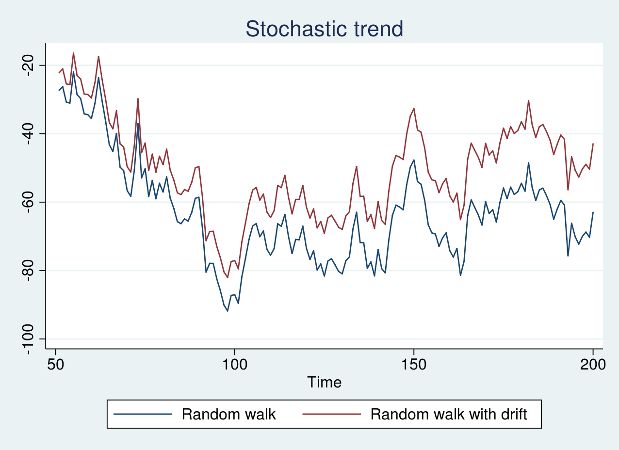
As seen in the graph above, there is no clear trend, and the red line appears to be shifted by a positive constant term from the blue line. If the series are graphed individually, it is impossible to distinguish whether the series are generated from a random walk or a random walk with drift. However, because both the series contain a stochastic trend, we can still apply differencing to achieve a stationary series.
Similarly, I generate simulated data from a random walk with a drift term of 1 and a deterministic time trend model and plot the graph below.
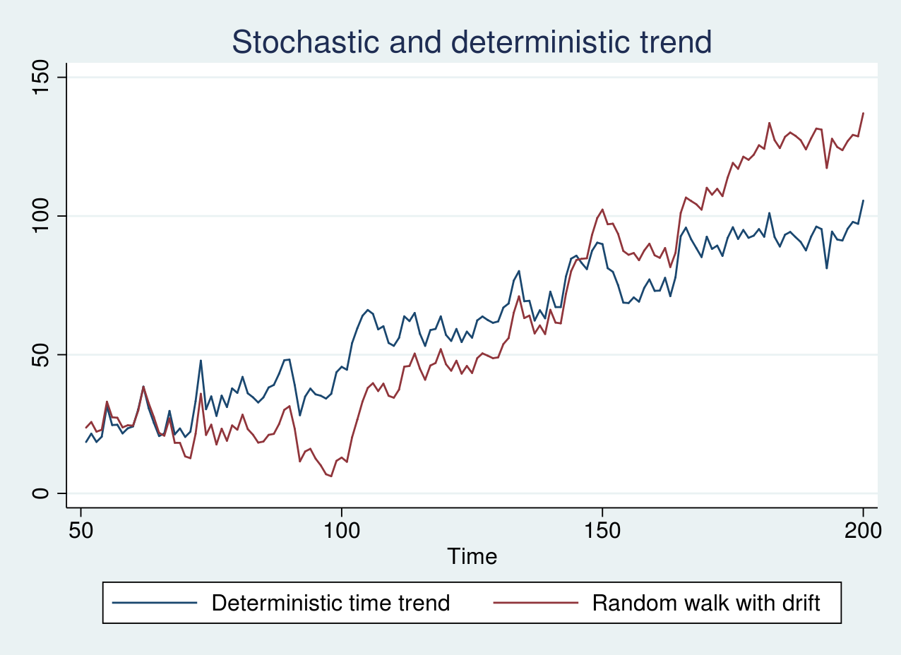
As seen in the graph above, the two series look remarkably similar. The blue line displays an erratic pattern around a constantly increasing trend line. The stochastic trend in the red line, however, increases slowly in the beginning of the sample and rapidly toward the end of the sample. In this case, it is crucial to apply the correct transformation as mentioned earlier.
Unit-root tests
Unit-root tests assume the null hypothesis that the true process is a random walk (1) or a random walk with a drift (2). Consider the following AR(1) model
\[
y_t = \phi y_{t-1} + \epsilon_t
\]
where \(\epsilon_t\) is independent and identically distributed with \(N(0,\sigma^2)\) distribution. The null hypothesis corresponds to \(\phi=1\), while the alternative is \(|\phi|<1\).
If \(\phi\) is indeed 1, as the sample size increases, the OLS estimator (\(\hat{\phi}\)) converges to the true value of 1 at a faster rate than it would if the process was stationary. However, the asymptotic distribution of \(\hat{\phi}\) is nonstandard, and the usual \(t\) tests become invalid.
Furthermore, depending on whether deterministic terms such as constants and time trends are included in the regression leads to different asymptotic distributions for the test statistic. This underscores the importance of clearly specifying the null as well as the alternative hypotheses while performing these tests.
Augmented Dickey–Fuller test
Under the null hypothesis, the true process is either a random walk or a random walk with drift. The Dickey–Fuller test involves fitting the model
\begin{equation}
\label{df}
y_t = \alpha + \delta t + \phi y_{t-1} + \epsilon_t \tag{3}
\end{equation}
The null hypothesis corresponds to \(\phi=1\). Estimating the parameters of (3) by OLS may fail to account for residual serial correlation. The augmented Dickey–Fuller (ADF) test addresses this by augmenting (3) by \(k\) number of lagged differences of the dependent variable. More specifically, it transforms (3) in difference form as
\begin{equation}
\label{adf}
\Delta y_t = \alpha + \delta t + \beta y_{t-1} + \sum_{i=1}^k \gamma_i \Delta y_{t-i} + \epsilon_t \tag{4}
\end{equation}
and tests whether \(\beta=0\). Note that (4) is in a general form and we can restrict \(\alpha\) or \(\delta\) or both to zero for regression specifications that lead to different distributions of the test statistic. Hamilton (1994, ch. 17) lists the distribution of the test statistic for four possible cases.
I begin by testing for a unit root in the series yrwd2 and yt, which correspond to data from a random walk with a drift term of 1 and a linear deterministic time trend model, respectively. I use dfuller to perform an ADF test. The null hypothesis I am interested in is that yrwd2 is a random walk process with a possible drift, while the alternative hypothesis posits that yrwd2 is stationary around a linear time trend. Hence, I use the option trend to control for a linear time trend in (4).
. dfuller yrwd2, trend

Dickey-Fuller test for unit root                 Number of obs   =       149

                             ---------- Interpolated Dickey-Fuller ---------
                  Test         1% Critical      5% Critical     10% Critical
               Statistic           Value            Value            Value
----------------------------------------------------------------------------
 Z(t)             -2.664            -4.024           -3.443           -3.143
----------------------------------------------------------------------------
MacKinnon approximate p-value for Z(t) = 0.2511
As expected, we fail to reject the null hypothesis of a random walk with a possible drift in yrwd2. Similarly, I test the presence of a unit root in the yt series.
. dfuller yt, trend

Dickey-Fuller test for unit root                 Number of obs   =       149

                             ---------- Interpolated Dickey-Fuller ---------
                  Test         1% Critical      5% Critical     10% Critical
               Statistic           Value             Value             Value
----------------------------------------------------------------------------
 Z(t)             -5.328            -4.024           -3.443           -3.143
----------------------------------------------------------------------------
MacKinnon approximate p-value for Z(t) = 0.0000
In this case, we reject the null hypothesis of a random walk with drift.
Phillips–Perron test
The tests developed in Phillips (1987) and Phillips and Perron (1988) modify the test statistics to account for the potential serial correlation and heteroskedasticity in the residuals. As in the Dickey–Fuller test, a regression model as in (3) is fit with OLS. The asymptotic distribution of the test statistics and critical values is the same as in the ADF test.
pperron performs a PP test in Stata and has a similar syntax as dfuller. Using pperron to test for a unit root in yrwd2 and yt yields a similar conclusion as the ADF test (output not shown here).
GLS detrended augmented Dickey–Fuller test
The GLS–ADF test proposed by Elliott et al. (1996) is similar to the ADF test. However, prior to fitting the model in (4), one first transforms the actual series via a generalized least-squares (GLS) regression. Elliott et al. (1996) show that this test has better power than the ADF test.
The null hypothesis is a random walk with a possible drift with two specific alternative hypotheses: the series is stationary around a linear time trend, or the series is stationary around a possible nonzero mean with no time trend.
To test whether the yrwd2 series is a random walk with drift, I use dfgls with a maximum of 4 lags for the regression specification in (4).
. dfgls yrwd2, maxlag(4)

DF-GLS for yrwd2                                      Number of obs =   145

               DF-GLS tau      1% Critical     5% Critical     10% Critical
  [lags]     Test Statistic        Value           Value            Value
---------------------------------------------------------------------------
    4            -1.404           -3.520          -2.930           -2.643
    3            -1.420           -3.520          -2.942           -2.654
    2            -1.638           -3.520          -2.953           -2.664
    1            -1.644           -3.520          -2.963           -2.673

Opt Lag (Ng-Perron seq t) = 0 [use maxlag(0)]
Min SC   =   3.31175 at lag  1 with RMSE  5.060941
Min MAIC =  3.295598 at lag  1 with RMSE  5.060941
Note that dfgls controls for a linear time trend by default unlike the dfuller or pperron command. We fail to reject the null hypothesis of a random walk with drift in the yrwd2 series.
Finally, I test the null hypothesis that yt is a random walk with drift using dfgls with a maximum of 4 lags.
. dfgls yt, maxlag(4)

DF-GLS for yt                                         Number of obs =   145

               DF-GLS tau      1% Critical     5% Critical     10% Critical
  [lags]     Test Statistic        Value           Value            Value
---------------------------------------------------------------------------
    4            -4.013           -3.520          -2.930           -2.643
    3            -4.154           -3.520          -2.942           -2.654
    2            -4.848           -3.520          -2.953           -2.664
    1            -4.844           -3.520          -2.963           -2.673

Opt Lag (Ng-Perron seq t) = 0 [use maxlag(0)]
Min SC   =  3.302146 at lag  1 with RMSE  5.036697
Min MAIC =  3.638026 at lag  1 with RMSE  5.036697
As expected, we reject the null hypothesis of a random walk with drift in the yt series.
Conclusion
In this post, I discussed nonstationary processes arising because of a stochastic trend, a deterministic time trend, or a combination of both. I illustrated the dfuller, pperron, and dfgls commands for testing the presence of a unit root using simulated data.
Appendix
The code for generating data from a random walk, random walk with drift, and linear deterministic trend models is provided below.
clear all
set seed 2016
local T = 200
set obs `T'
gen time = _n
label var time "Time"
tsset time
gen eps = rnormal(0,5)

/*Random walk*/
gen yrw = eps in 1
replace yrw = l.yrw + eps in 2/l

/*Random walk with drift*/
gen yrwd1 = 0.1 + eps in 1
replace yrwd1 = 0.1 + l.yrwd1 + eps in 2/l

/*Random walk with drift*/
gen yrwd2 = 1 + eps in 1
replace yrwd2 = 1 + l.yrwd2 + eps in 2/l

/*Stationary around a time trend model*/
gen yt = 0.5 + 0.1*time + eps in 1
replace yt = 0.5 + 0.1*time +0.8*l.yt+ eps in 2/l
drop in 1/50

tsline yrw yrwd1, title("Stochastic trend")          ///
        legend(label(1 "Random walk")                ///
        label(2 "Random walk with drift"))
tsline yt yrwd2,                                     ///
        legend(label(1 "Deterministic time trend")   ///
        label(2 "Random walk with drift"))           ///
        title("Stochastic and deterministic trend")
Lines 1–4 clear the current Stata session, set the seed for the random number generator, define a local macro T as the number of observations, and set it to 200. Lines 5–7 generate the time variable and declare it as a time series. Line 8 generates a zero mean random normal error with standard deviation 5. Lines 10–12 generate data from a random walk model and store them in the variable yrw. Lines 14–16 generate data from a random walk with a drift of 0.1 and store them in the variable yrwd1. Lines 18–20 generate data from a random walk with a drift of 1 and store in the variable yrwd2. Lines 22–24 generate data from a deterministic time trend model and store them in the variable yt. Line 25 drops the first 50 observations as burn-in. Lines 27–33 plot the time series.
References
Elliott, G. R., T. J. Rothenberg, and J. H. Stock. 1996. Efficient tests for an autoregressive unit root. Econometrica 64: 813–836.
Hamilton, J. D. 1994. Time Series Analysis. Princeton: Princeton University Press.
Phillips, P. C. B. 1987. Time series regression with a unit root. Econometrica 55: 277–301.
Phillips, P. C. B., and P. Perron. 1988. Testing for a unit root in time series regression. Biometrika 75: 335–346.