Group comparisons in structural equation models: Testing measurement invariance
When fitting almost any model, we may be interested in investigating whether parameters differ across groups such as time periods, age groups, gender, or school attended. In other words, we may wish to perform tests of moderation when the moderator variable is categorical. For regression models, this can be as simple as including group indicators in the model and interacting them with other predictors.
We naturally have hypotheses regarding differences in parameters across groups when fitting structural equation models as well. When these models involve latent variables and the corresponding observed measurements, we can test whether those measurements are invariant across groups. Evaluation of measurement invariance typically involves a series of tests for equality of measurement coefficients (factor loadings), equality of intercepts, and equality of error variances across groups.
In this post, I demonstrate how to use the sem command’s group() and ginvariant() options as well as the postestimation command estat ginvariant to easily perform tests of measurement invariance.
Measurement invariance example
I use data from Holzinger and Swineford (1939), which records students’ scores on a number of exams designed to measure different types of abilities. The students in this dataset came from two different schools, the Pasteur school and the Grant-White school, and I want to test for differences across schools. Here I focus on three exams that were intended to measure spatial abilities. I will fit the confirmatory factor model corresponding to the following path diagram and perform a series of tests for measurement invariance. Although this example uses the sem command, I could have equivalently drawn this diagram in the Builder and selected group analysis to fit all the models discussed below.
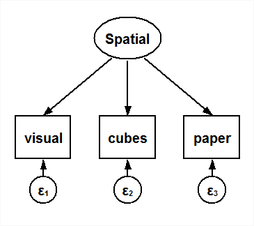
To begin, I fit a model with all parameters estimated separately across groups. There are various ways to set the required identifying constraints that provide a scale and location for the latent variable. Here I set the mean of the Spatial latent variable to 0 and the variance to 1 in both groups.
. sem (Spatial -> visual cubes paper),
> variance(Spatial@1) mean(Spatial@0) ginvariant(none) group(school)

Endogenous variables

Measurement:  visual cubes paper

Exogenous variables

Latent:       Spatial

Fitting target model:

Iteration 0:   log likelihood = -2603.5782
Iteration 1:   log likelihood = -2603.5782

Structural equation model                       Number of obs     =        301
Grouping variable  = school                     Number of groups  =          2
Estimation method  = ml
Log likelihood     = -2603.5782

 ( 1)  [var(Spatial)]1bn.school = 1
 ( 2)  [mean(Spatial)]1bn.school = 0
 ( 3)  [var(Spatial)]2.school = 1
 ( 4)  [mean(Spatial)]2.school = 0
-------------------------------------------------------------------------------
              |                 OIM
              |      Coef.   Std. Err.      z    P>|z|     [95% Conf. Interval]
--------------+----------------------------------------------------------------
Measurement   |
  visual <-   |
      Spatial |
     Pasteur  |   4.264065   .8600633     4.96   0.000     2.578372    5.949759
  Grant-Wh~e  |    5.49895   1.190435     4.62   0.000     3.165739     7.83216
        _cons |
     Pasteur  |   29.64744   .5674293    52.25   0.000     28.53529    30.75958
  Grant-Wh~e  |   29.57931   .5721785    51.70   0.000     28.45786    30.70076
  ------------+----------------------------------------------------------------
  cubes <-    |
      Spatial |
     Pasteur  |    2.26321   .5214501     4.34   0.000     1.241187    3.285234
  Grant-Wh~e  |   1.808245   .5031516     3.59   0.000     .8220861    2.794404
        _cons |
     Pasteur  |    23.9359   .3927222    60.95   0.000     23.16618    24.70562
  Grant-Wh~e  |       24.8   .3678649    67.42   0.000       24.079      25.521
  ------------+----------------------------------------------------------------
  paper <-    |
      Spatial |
     Pasteur  |   1.695466   .3429472     4.94   0.000     1.023302     2.36763
  Grant-Wh~e  |   1.311235   .3413206     3.84   0.000     .6422592    1.980211
        _cons |
     Pasteur  |   14.16026    .227089    62.36   0.000     13.71517    14.60534
  Grant-Wh~e  |   14.30345   .2335324    61.25   0.000     13.84573    14.76116
--------------+----------------------------------------------------------------
 mean(Spatial)|
          [*] |          0  (constrained)
--------------+----------------------------------------------------------------
 var(e.visual)|
     Pasteur  |   32.04601   6.912718                       20.9971    48.90898
 Grant-White  |   17.23285   12.18676                      4.309258    68.91467
  var(e.cubes)|
     Pasteur  |   18.93787   2.710244                      14.30585    25.06967
 Grant-White  |   16.35232   2.318816                      12.38443    21.59149
  var(e.paper)|
     Pasteur  |   5.170226    1.09911                      3.408453    7.842631
 Grant-White  |   6.188581   .9975804                      4.512114    8.487938
  var(Spatial)|
          [*] |          1  (constrained)
-------------------------------------------------------------------------------
Note: [*] identifies parameter estimates constrained to be equal across groups.
LR test of model vs. saturated: chi2(0)   =      0.00, Prob > chi2 =      .
Glancing through this output, we see that many of the parameter estimates are very similar for the two schools. The estat ginvariant command provides tests of invariance across groups.
. estat ginvariant, showpclass(mcoef) class

Tests for group invariance of parameters

------------------------------------------------------------------------------
             |            Wald Test                       Score Test
             |      chi2         df    p>chi2       chi2          df    p>chi2
-------------+----------------------------------------------------------------
Measurement  |
  visual <-  |
     Spatial |     0.707          1    0.4004          .           .         .
  -----------+----------------------------------------------------------------
  cubes <-   |
     Spatial |     0.394          1    0.5301          .           .         .
  -----------+----------------------------------------------------------------
  paper <-   |
     Spatial |     0.631          1    0.4271          .           .         .
------------------------------------------------------------------------------

Joint tests for each parameter class

------------------------------------------------------------------------------
             |            Wald Test                       Score Test
             |      chi2         df    p>chi2       chi2          df    p>chi2
-------------+----------------------------------------------------------------
       mcoef |     1.097          3    0.7778          .           .         .
------------------------------------------------------------------------------
The showpclass(mcoef) and class options restricted the results to tests regarding measurement coefficients and requested a joint test for the hypothesis that all measurement coefficients are equal across groups. The first table in the output reports separate tests of equality of the measurement coefficients across groups. My focus now, however, is on the joint Wald test shown in the second table, and we fail to reject the hypothesis of equality across groups for all measurement coefficients.
I now include the ginvariant(mcoef) option in order to fit a model with the measurement coefficients constrained to be equal across groups by typing
. sem (Spatial -> visual cubes paper), variance(Spatial@1) ///
       mean(Spatial@0) ginvariant(mcoef) group(school)
and then test whether the intercepts can be constrained:
. estat ginvariant, showpclass(mcons) class

Tests for group invariance of parameters

------------------------------------------------------------------------------
             |            Wald Test                       Score Test
             |      chi2         df    p>chi2       chi2          df    p>chi2
-------------+----------------------------------------------------------------
Measurement  |
  visual <-  |
       _cons |     0.007          1    0.9326          .           .         .
  -----------+----------------------------------------------------------------
  cubes <-   |
       _cons |     2.580          1    0.1082          .           .         .
  -----------+----------------------------------------------------------------
  paper <-   |
       _cons |     0.193          1    0.6605          .           .         .
------------------------------------------------------------------------------

Joint tests for each parameter class

------------------------------------------------------------------------------
             |            Wald Test                       Score Test
             |      chi2         df    p>chi2       chi2          df    p>chi2
-------------+----------------------------------------------------------------
       mcons |     3.011          3    0.3900          .           .         .
------------------------------------------------------------------------------
We fail to reject the null hypothesis that all intercepts are equal across groups, so I fit the model with those equality constraints by specifying the ginvariant(mcoef mcons) option.
. sem (Spatial -> visual cubes paper), variance(Spatial@1) ///
      mean(Spatial@0) ginvariant(mcoef mcons) group(school)
Then, I test the equality of the error variances.
. estat ginvariant, showpclass(merrvar) class

Tests for group invariance of parameters

------------------------------------------------------------------------------
             |            Wald Test                       Score Test
             |      chi2         df    p>chi2       chi2          df    p>chi2
-------------+----------------------------------------------------------------
var(e.visual)|     0.359          1    0.5493          .           .         .
 var(e.cubes)|     1.413          1    0.2345          .           .         .
 var(e.paper)|     0.014          1    0.9052          .           .         .
------------------------------------------------------------------------------

Joint tests for each parameter class

------------------------------------------------------------------------------
             |            Wald Test                       Score Test
             |      chi2         df    p>chi2       chi2          df    p>chi2
-------------+----------------------------------------------------------------
     merrvar |     1.857          3    0.6027          .           .         .
------------------------------------------------------------------------------
Once again, we fail to reject the null hypothesis of invariance across groups. I now impose constraints on the coefficients, intercepts, and error variances while allowing the mean and variance of the latent variable to differ across groups. To do this, I remove the mean(Spatial@0) option and replace the variance(Spatial@1) with variance(1:Spatial@1). With this change, the mean and variance of Spatial will be set to 0 and 1, respectively, in the first group but estimated freely in the second group.
. sem (Spatial -> visual cubes paper),
> variance(1:Spatial@1) ginvariant(mcoef mcons merrvar) group(school)

Endogenous variables

Measurement:  visual cubes paper

Exogenous variables

Latent:       Spatial

Fitting target model:

Iteration 0:   log likelihood = -5357.6935  (not concave)
Iteration 1:   log likelihood = -4792.5814  (not concave)
Iteration 2:   log likelihood = -4316.3827  (not concave)
Iteration 3:   log likelihood =  -2769.069  (not concave)
Iteration 4:   log likelihood = -2662.2605
Iteration 5:   log likelihood = -2645.7652
Iteration 6:   log likelihood = -2629.1987
Iteration 7:   log likelihood =   -2622.83  (not concave)
Iteration 8:   log likelihood = -2622.3555
Iteration 9:   log likelihood = -2622.3227
Iteration 10:  log likelihood = -2621.9007
Iteration 11:  log likelihood = -2621.8931
Iteration 12:  log likelihood =  -2621.893

Structural equation model                       Number of obs     =        301
Grouping variable  = school                     Number of groups  =          2
Estimation method  = ml
Log likelihood     =  -2621.893

 ( 1)  [cubes]1bn.school#c.Spatial - [cubes]2.school#c.Spatial = 0
 ( 2)  [paper]1bn.school#c.Spatial - [paper]2.school#c.Spatial = 0
 ( 3)  [var(e.visual)]1bn.school - [var(e.visual)]2.school = 0
 ( 4)  [var(e.cubes)]1bn.school - [var(e.cubes)]2.school = 0
 ( 5)  [var(e.paper)]1bn.school - [var(e.paper)]2.school = 0
 ( 6)  [var(Spatial)]1bn.school = 1
 ( 7)  [visual]1bn.school - [visual]2.school = 0
 ( 8)  [cubes]1bn.school - [cubes]2.school = 0
 ( 9)  [paper]1bn.school - [paper]2.school = 0
 (10)  [visual]2.school#c.Spatial = 1
 (11)  [mean(Spatial)]1bn.school = 0
-------------------------------------------------------------------------------
              |                 OIM
              |      Coef.   Std. Err.      z    P>|z|     [95% Conf. Interval]
--------------+----------------------------------------------------------------
Measurement   |
  visual <-   |
      Spatial |
     Pasteur  |   5.472561   1.129916     4.84   0.000     3.257966    7.687156
  Grant-Wh~e  |          1  (constrained)
        _cons |
          [*] |   29.32102   .4932735    59.44   0.000     28.35422    30.28782
  ------------+----------------------------------------------------------------
  cubes <-    |
      Spatial |
          [*] |   .3968564   .1833049     2.17   0.030     .0375854    .7561274
        _cons |
          [*] |   24.26618   .2890016    83.97   0.000     23.69975    24.83262
  ------------+----------------------------------------------------------------
  paper <-    |
      Spatial |
          [*] |   .2953686    .137265     2.15   0.031     .0263341    .5644031
        _cons |
          [*] |   14.16525   .1786194    79.30   0.000     13.81516    14.51533
--------------+----------------------------------------------------------------
 mean(Spatial)|
     Pasteur  |          0  (constrained)
 Grant-White  |   .4140109   .6928933     0.60   0.550    -.9440351    1.772057
--------------+----------------------------------------------------------------
 var(e.visual)|
          [*] |   19.50062   12.09195                      5.784095    65.74481
  var(e.cubes)|
          [*] |   20.08682   1.784905                      16.87617    23.90829
  var(e.paper)|
          [*] |   6.864085    .691005                      5.634982    8.361281
  var(Spatial)|
     Pasteur  |          1  (constrained)
 Grant-White  |   25.44848   15.33031                      7.814351    82.87636
-------------------------------------------------------------------------------
Note: [*] identifies parameter estimates constrained to be equal across groups.
LR test of model vs. saturated: chi2(7)   =     36.63, Prob > chi2 = 0.0000
The mean of 0.414 for Spatial in the Grant-White school represents the difference in means of this latent variable across schools, and we find the difference in means across schools is not significantly different from 0.
Summary
Tests of hypotheses regarding the equality of parameters across groups are easily performed using the sem command and estat ginvariant. While there are minor variations throughout structural equation modeling literature in recommendations for setting identifying constraints and for the order of tests for invariance, the tools that I have demonstrated can be adapted to accommodate any form of tests for measurement invariance. These same tools can also be used to test for parameter invariance across groups in other types of structural equation models.
Reference
Holzinger, K.~J., and F. Swineford. 1939. A study in factor analysis: The stability of a bi-factor solution. Supplementary Educational Monographs, 48. Chicago, IL: University of Chicago.