xtmixed was built from the ground up for dealing with multilevel random effects — that is its raison d’être. sem was built for multivariate outcomes, for handling latent variables, and for estimating structural equations (also called simultaneous systems or models with endogeneity). Can sem also handle multilevel random effects (REs)? Do we care?

This would be a short entry if either answer were “no”, so let’s get after the first question.

Can sem handle multilevel REs?

A good place to start is to simulate some multilevel RE data. Let’s create data for the 3-level regression model

where the classical multilevel regression assumption holds that and are distributed normal and are uncorrelated.

This represents a model of nested within nested within . An example would be students nested within schools nested within counties. We have random intercepts at the 2nd and 3rd levels — , . Because these are random effects, we need estimate only the variance of , , and .

For our simulated data, let’s assume there are 3 groups at the 3rd level, 2 groups at the 2nd level within each 3rd level group, and 2 individuals within each 2nd level group. Or, , , and . Having only 3 groups at the 3rd level is silly. It gives us only 3 observations to estimate the variance of . But with only observations, we will be able to easily see our entire dataset, and the concepts scale to any number of 3rd-level groups.

First, create our 3rd-level random effects — .

. set obs 3
. gen k = _n
. gen Uk = rnormal()

There are only 3 in our dataset.

I am showing the effects symbolically in the table rather than showing numeric values. It is the pattern of unique effects that will become interesting, not their actual values.

Now, create our 2nd-level random effects — — by doubling this data and creating 2nd-level effects.

. expand 2
. by k, sort: gen j = _n
. gen Vjk = rnormal()

We have 6 unique values of our 2nd-level effects and the same 3 unique values of our 3rd-level effects. Our original 3rd-level effects just appear twice each.

Now, create our 1st-level random effects — — which we typically just call errors.

. expand 2
. by k j, sort: gen i = _n
. gen Eijk = rnormal()

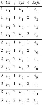
There are still only 3 unique in our dataset, and only 6 unique .

Finally, we create our regression data, using ,

. gen xijk = runiform()
. gen yijk = 2 * xijk + Uk + Vjk + Eijk

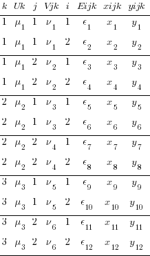
We could estimate our multilevel RE model on this data by typing,

. xtmixed yijk xijk || k: || j:

xtmixed uses the index variables k and j to deeply understand the multilevel structure of the our data. sem has no such understanding of multilevel data. What it does have is an understanding of multivariate data and a comfortable willingness to apply constraints.

Let’s restructure our data so that sem can be made to understand its multilevel structure.

First some renaming so that the results of our restructuring will be easier to interpret.

. rename Uk U
. rename Vjk V
. rename Eijk E
. rename xijk x
. rename yijk y

We reshape to turn our multilevel data into multivariate data that sem has a chance of understanding. First, we reshape wide on our 2nd-level identifier j. Before that, we egen to create a unique identifier for each observation of the two groups identified by j.

. egen ik = group(i k)
. reshape wide y x E V, i(ik) j(j)

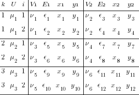
We now have a y variable for each group in j (y1 and y2). Likewise, we have two x variables, two residuals, and most importantly two 2nd-level random effects V1 and V2. This is the same data, we have merely created a set of variables for every level of j. We have gone from multilevel to multivariate.
We still have a multilevel component. There are still two levels of i in our dataset. We must reshape wide again to remove any remnant of multilevel structure.

. drop ik
. reshape wide y* x* E*, i(k) j(i)

I admit that is a microscopic font, but it is the structure that is important, not the values. We now have 4 y’s, one for each combination of 2nd- and 3rd-level identifiers — i and j. Likewise for the x’s and E’s.

We can think of each xji yji pair of columns as representing a regression for a specific combination of j and i — y11 on x11, y12 on x12, y21 on x21, and y22 on x22. Or, more explicitly,

So, rather than a univariate multilevel regression with 4 nested observation sets, () * (), we now have 4 regressions which are all related through and each of two pairs are related through . Oh, and all share the same coefficient . Oh, and the all have identical variances. Oh, and the also have identical variances. Luckily both the sem command and the SEM Builder (the GUI for sem) make setting constraints easy.

There is one other thing we haven’t addressed. xtmixed understands random effects. Does sem? Random effects are just unobserved (latent) variables and sem clearly understands those. So, yes, sem does understand random effects.

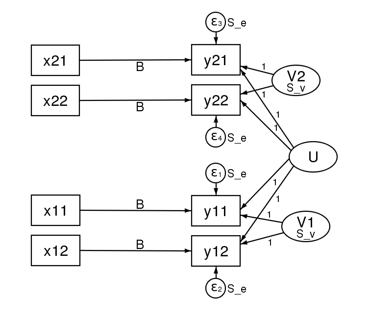
Many SEMers would represent this model in a path diagram by drawing.

There is a lot of information in that diagram. Each regression is represented by one of the x boxes being connected by a path to a y box. That each of the four paths is labeled with means that we have constrained the regressions to have the same coefficient. The y21 and y22 boxes also receive input from the random latent variable V2 (representing our 2nd-level random effects). The other two y boxes receive input from V1 (also our 2nd-level random effects). For this to match how xtmixed handles random effects, V1 and V2 must be constrained to have the same variance. This was done in the path diagram by “locking” them to have the same variance — S_v. To match xtmixed, each of the four residuals must also have the same variance — shown in the diagram as S_e. The residuals and random effect variables also have their paths constrained to 1. That is to say, they do not have coefficients.

We do not need any of the U, V, or E variables. We kept these only to make clear how the multilevel data was restructured to multivariate data. We might “follow the money” in a criminal investigation, but with simulated multilevel data is is best to “follow the effects”. Seeing how these effects were distributed in our reshaped data made it clear how they entered our multivariate model.

Just to prove that this all works, here are the results from a simulated dataset ( rather than the 3 that we have been using). The xtmixed results are,

. xtmixed yijk xijk || k: || j: , mle var

  (log omitted)

Mixed-effects ML regression                     Number of obs      =       400

-----------------------------------------------------------
                |   No. of       Observations per Group
 Group Variable |   Groups    Minimum    Average    Maximum
----------------+------------------------------------------
              k |      100          4        4.0          4
              j |      200          2        2.0          2
-----------------------------------------------------------

                                                Wald chi2(1)       =     61.84
Log likelihood = -768.96733                     Prob > chi2        =    0.0000

------------------------------------------------------------------------------
        yijk |      Coef.   Std. Err.      z    P>|z|     [95% Conf. Interval]
-------------+----------------------------------------------------------------
        xijk |   1.792529   .2279392     7.86   0.000     1.345776    2.239282
       _cons |    .460124   .2242677     2.05   0.040     .0205673    .8996807
------------------------------------------------------------------------------

------------------------------------------------------------------------------
  Random-effects Parameters  |   Estimate   Std. Err.     [95% Conf. Interval]
-----------------------------+------------------------------------------------
k: Identity                  |
                  var(_cons) |   2.469012   .5386108      1.610034    3.786268
-----------------------------+------------------------------------------------
j: Identity                  |
                  var(_cons) |   1.858889    .332251      1.309522    2.638725
-----------------------------+------------------------------------------------
               var(Residual) |   .9140237   .0915914      .7510369    1.112381
------------------------------------------------------------------------------
LR test vs. linear regression:       chi2(2) =   259.16   Prob > chi2 = 0.0000

Note: LR test is conservative and provided only for reference.

The sem results are,

sem (y11 <- x11@bx _cons@c V1@1 U@1)
    (y12 <- x12@bx _cons@c V1@1 U@1)
    (y21 <- x21@bx _cons@c V2@1 U@1)
    (y22 <- x22@bx _cons@c V2@1 U@1) ,
        covstruct(_lexog, diagonal) cov(_lexog*_oexog@0)  
        cov( V1@S_v V2@S_v  e.y11@S_e e.y12@S_e e.y21@S_e e.y22@S_e)
  
  (notes omitted)

Endogenous variables

Observed:  y11 y12 y21 y22

Exogenous variables

Observed:  x11 x12 x21 x22
Latent:    V1 U V2
  
  (iteration log omitted)

Structural equation model                       Number of obs      =       100
Estimation method  = ml
Log likelihood     = -826.63615
  
  (constraint listing omitted)
------------------------------------------------------------------------------
             |                 OIM             |      Coef.   Std. Err.      z    P>|z|     [95% Conf. Interval]
-------------+----------------------------------------------------------------
Structural   |  
  y11 <-     |
         x11 |   1.792529   .2356323     7.61   0.000     1.330698     2.25436
          V1 |          1   7.68e-17  1.3e+16   0.000            1           1
           U |          1   2.22e-18  4.5e+17   0.000            1           1
       _cons |    .460124    .226404     2.03   0.042     .0163802    .9038677
  -----------+----------------------------------------------------------------
  y12 <-     |
         x12 |   1.792529   .2356323     7.61   0.000     1.330698     2.25436
          V1 |          1   2.00e-22  5.0e+21   0.000            1           1
           U |          1   5.03e-17  2.0e+16   0.000            1           1
       _cons |    .460124    .226404     2.03   0.042     .0163802    .9038677
  -----------+----------------------------------------------------------------
  y21 <-     |
         x21 |   1.792529   .2356323     7.61   0.000     1.330698     2.25436
           U |          1   5.70e-46  1.8e+45   0.000            1           1
          V2 |          1   5.06e-45  2.0e+44   0.000            1           1
       _cons |    .460124    .226404     2.03   0.042     .0163802    .9038677
  -----------+----------------------------------------------------------------
  y22 <-     |
         x22 |   1.792529   .2356323     7.61   0.000     1.330698     2.25436
           U |          1  (constrained)
          V2 |          1  (constrained) 
       _cons |    .460124    .226404     2.03   0.042     .0163802    .9038677
-------------+----------------------------------------------------------------
Variance     |
       e.y11 |   .9140239    .091602                        .75102    1.112407
       e.y12 |   .9140239    .091602                        .75102    1.112407
       e.y21 |   .9140239    .091602                        .75102    1.112407
       e.y22 |   .9140239    .091602                        .75102    1.112407
          V1 |   1.858889   .3323379                      1.309402    2.638967
           U |   2.469011   .5386202                      1.610021    3.786296
          V2 |   1.858889   .3323379                      1.309402    2.638967
-------------+----------------------------------------------------------------
Covariance   |
  x11        |
          V1 |          0  (constrained)
           U |          0  (constrained)
          V2 |          0  (constrained)
  -----------+----------------------------------------------------------------
  x12        |
          V1 |          0  (constrained)
           U |          0  (constrained)
          V2 |          0  (constrained)
  -----------+----------------------------------------------------------------
  x21        |
          V1 |          0  (constrained)
           U |          0  (constrained)
          V2 |          0  (constrained)
  -----------+----------------------------------------------------------------
  x22        |
          V1 |          0  (constrained)
           U |          0  (constrained)
          V2 |          0  (constrained)
  -----------+----------------------------------------------------------------
  V1         |
           U |          0  (constrained)
          V2 |          0  (constrained)
  -----------+----------------------------------------------------------------
  U          |
          V2 |          0  (constrained)
------------------------------------------------------------------------------
LR test of model vs. saturated: chi2(25)  =     22.43, Prob > chi2 = 0.6110

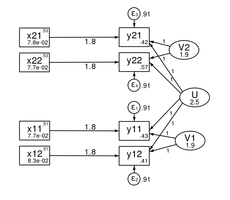
And here is the path diagram after estimation.

The standard errors of the two estimation methods are asymptotically equivalent, but will differ in finite samples.

Sidenote: Those familiar with multilevel modeling will be wondering if sem can handle unbalanced data. That is to say a different number of observations or subgroups within groups. It can. Simply let reshape create missing values where it will and then add the method(mlmv) option to your sem command. mlmv stands for maximum likelihood with missing values. And, as strange as it may seem, with this option the multivariate sem representation and the multilevel xtmixed representations are the same.

Do we care?

You will have noticed that the sem command was, well, it was really long. (I wrote a little loop to get all the constraints right.) You will also have noticed that there is a lot of redundant output because our SEM model has so many constraints. Why would anyone go to all this trouble to do something that is so simple with xtmixed? The answer lies in all of those constraints. With sem we can relax any of those constraints we wish!

Relax the constraint that the V# have the same variance and you can introduce heteroskedasticity in the 2nd-level effects. That seems a little silly when there are only two levels, but imagine there were 10 levels.

Add a covariance between the V# and you introduce correlation between the groups in the 3rd level.

What’s more, the pattern of heteroskedasticity and correlation can be arbitrary. Here is our path diagram redrawn to represent children within schools within counties and increasing the number of groups in the 2nd level.

We have 5 counties at the 3rd level and two schools within each county at the 2nd level — for a total of 10 dimensions in our multivariate regression. The diagram does not change based on the number of children drawn from each school.

Our regression coefficients have been organized horizontally down the center of the diagram to allow room along the left and right for the random effects. Taken as a multilevel model, we have only a single covariate — x. Just to be clear, we could generalize this to multiple covariates by adding more boxes with covariates for each dependent variable in the diagram.

The labels are chosen carefully. The 3rd-level effects N1, N2, and N3 are for northern counties, and the remaining second level effects S1 and S2 are for southern counties. There is a separate dependent variable and associated error for each school. We have 4 public schools (pub1 pub2, pub3, and pub4); three private schools (prv1 prv2, and prv3); and 3 church-sponsored schools (chr1 chr2, and chr3).

The multivariate structure seen in the diagram makes it clear that we can relax some constraints that the multilevel model imposes. Because the sem representation of the model breaks the 2nd level effect into an effect for each county, we can apply a structure to the 2nd level effect. Consider the path diagram below.

We have correlated the effects for the 3 northern counties. We did this by drawing curved lines between the effects. We have also correlated the effects of the two southern counties. xtmixed does not allow these types of correlations. Had we wished, we could have constrained the correlations of the 3 northern counties to be the same.

We could also have allowed the northern and southern counties to have different variances. We did just that in the diagram below by constraining the northern counties variances to be N and the southern counties variances to be S.

In this diagram we have also correlated the errors for the 4 public schools. As drawn, each correlation is free to take on its own values, but we could just as easily constrain each public school to be equally correlated with all other public schools. Likewise, to keep the diagram readable, we did not correlate the private schools with each other or the church schools with each other. We could have done that.

There is one thing that xtmixed can do that sem cannot. It can put a structure on the residual correlations within the 2nd level groups. xtmixed has a special option, residuals(), for just this purpose.

With xtmixed and sem you get,

• robust and cluster-robust SEs
• survey data

With sem you also get

• endogenous covariates
• estimation by GMM
• missing data — MAR (also called missing on observables)
• heteroskedastic effects at any level
• correlated effects at any level
• easy score tests using estat scoretests
  • are the coefficients truly are the same across all equations/levels, whether effects?
  • are effects or sets of effects uncorrelated?
  • are effects within a grouping homoskedastic?
  • …

Whether you view this rethinking of multilevel random-effects models as multivariate structural equation models (SEMs) as interesting, or merely an academic exercise, depends on whether your model calls for any of the items in the second list.