Using Stata’s SEM features to model the Beck Depression Inventory
I just got back from the 2012 Stata Conference in San Diego where I gave a talk on Psychometric Analysis Using Stata and from the 2012 American Psychological Association Meeting in Orlando. Stata’s structural equation modeling (SEM) builder was popular at both meetings and I wanted to show you how easy it is to use. If you are not familiar with the basics of SEM, please refer to the references at the end of the post. My goal is simply to show you how to use the SEM builder assuming that you already know something about SEM. If you would like to view a video demonstration of the SEM builder, please click the play button below:
The data used here and for the silly examples in my talk were simulated to resemble one of the most commonly used measures of depression: the Beck Depression Inventory (BDI). If you find these data too silly or not relevant to your own research, you could instead imagine it being a set of questions to measure mathematical ability, the ability to use a statistical package, or whatever you wanted.
The Beck Depression Inventory
Originally published by Aaron Beck and colleagues in 1961, the BDI marked an important change in the conceptualization of depression from a psychoanalytic perspective to a cognitive/behavioral perspective. It was also a landmark in the measurement of depression shifting from lengthy, expensive interviews with a psychiatrist to a brief, inexpensive questionnaire that could be scored and quantified. The original inventory consisted of 21 questions each allowing ordinal responses of increasing symptom severity from 0-3. The sum of the responses could then be used to classify a respondent’s depressive symptoms as none, mild, moderate or severe. Many studies have demonstrated that the BDI has good psychometric properties such as high test-retest reliability and the scores correlate well with the assessments of psychiatrists and psychologists. The 21 questions can also be grouped into two subscales. The affective scale includes questions like “I feel sad” and “I feel like a failure” that quantify emotional symptoms of depression. The somatic or physical scale includes questions like “I have lost my appetite” and “I have trouble sleeping” that quantify physical symptoms of depression. Since its original publication, the BDI has undergone two revisions in response to the American Psychiatric Association’s (APA) Diagnostic and Statistical Manuals (DSM) and the BDI-II remains very popular.
The Stata Depression Inventory
Since the BDI is a copyrighted psychometric instrument, I created a fictitious instrument called the “Stata Depression Inventory”. It consists of 20 questions each beginning with the phrase “My statistical software makes me…”. The individual questions are listed in the variable labels below.
. describe qu1-qu20

variable  storage  display    value
 name       type   format     label      variable label
------------------------------------------------------------------------------
qu1         byte   %16.0g     response   ...feel sad
qu2         byte   %16.0g     response   ...feel pessimistic about the future
qu3         byte   %16.0g     response   ...feel like a failure
qu4         byte   %16.0g     response   ...feel dissatisfied
qu5         byte   %16.0g     response   ...feel guilty or unworthy
qu6         byte   %16.0g     response   ...feel that I am being punished
qu7         byte   %16.0g     response   ...feel disappointed in myself
qu8         byte   %16.0g     response   ...feel am very critical of myself
qu9         byte   %16.0g     response   ...feel like harming myself
qu10        byte   %16.0g     response   ...feel like crying more than usual
qu11        byte   %16.0g     response   ...become annoyed or irritated easily
qu12        byte   %16.0g     response   ...have lost interest in other people
qu13        byte   %16.0g     qu13_t1    ...have trouble making decisions
qu14        byte   %16.0g     qu14_t1    ...feel unattractive
qu15        byte   %16.0g     qu15_t1    ...feel like not working
qu16        byte   %16.0g     qu16_t1    ...have trouble sleeping
qu17        byte   %16.0g     qu17_t1    ...feel tired or fatigued
qu18        byte   %16.0g     qu18_t1    ...makes my appetite lower than usual
qu19        byte   %16.0g     qu19_t1    ...concerned about my health
qu20        byte   %16.0g     qu20_t1    ...experience decreased libido
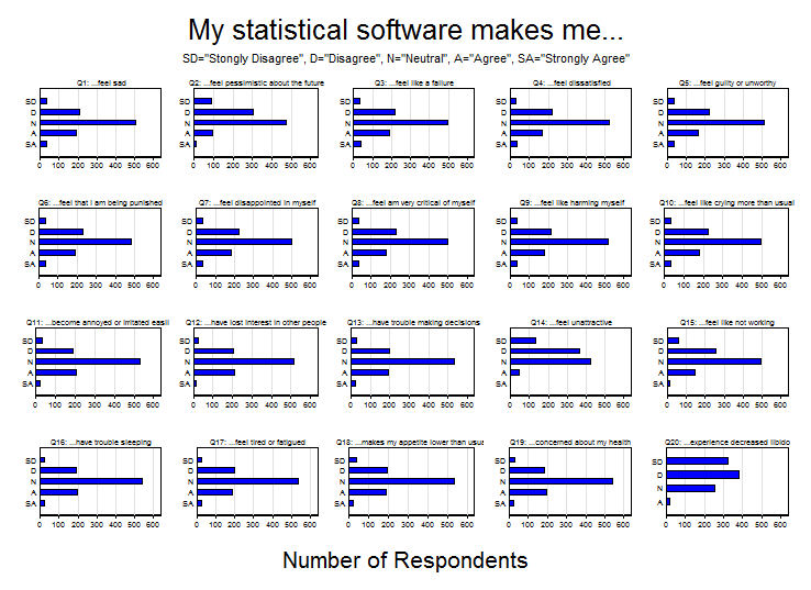
The responses consist of a 5-point Likert scale ranging from 1 (Strongly Disagree) to 5 (Strongly Agree). Questions 1-10 form the affective scale of the inventory and questions 11-20 form the physical scale. Data were simulated for 1000 imaginary people and included demographic variables such as age, sex and race. The responses can be summarized succinctly in a matrix of bar graphs:
Classical statistical analysis
The beginning of a classical statistical analysis of these data might consist of summing the responses for questions 1-10 and referring to them as the “Affective Depression Score” and summing questions 11-20 and referring to them as the “Physical Depression Score”.
egen Affective = rowtotal(qu1-qu10)
label var Affective "Affective Depression Score"
egen physical = rowtotal(qu11-qu20)
label var physical "Physical Depression Score"
We could be more sophisticated and use principal components to create the affective and physical depression score:
pca qu1-qu20, components(2)
predict Affective Physical
label var Affective "Affective Depression Score"
label var Physical "Physical Depression Score"
We could then ask questions such as “Are there differences in affective and physical depression scores by sex?” and test these hypotheses using multivariate statistics such as Hotelling’s T-squared statistic. The problem with this analysis strategy is that it treats the depression scores as though they were measured without error and can lead to inaccurate p-values for our test statistics.
Structural equation modeling
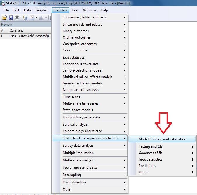
Structural equation modeling (SEM) is an ideal way to analyze data where the outcome of interest is a scale or scales derived from a set of measured variables. The affective and physical scores are treated as latent variables in the model resulting in accurate p-values and, best of all….these models are very easy to fit using Stata! We begin by selecting the SEM builder from the Statistics menu:
In the SEM builder, we can select the “Add Measurement Component” icon:
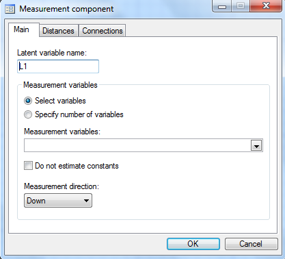
which will open the following dialog box:
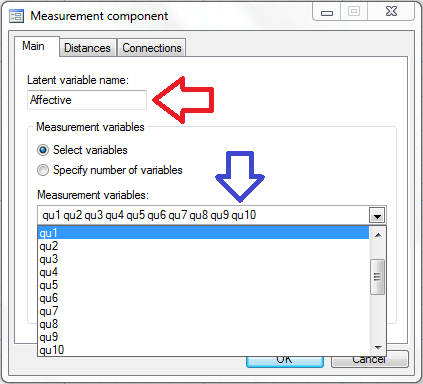
In the box labeled “Latent Variable Name” we can type “Affective” (red arrow below) and we can select the variables qu1-qu10 in the “Measured variables” box (blue arrow below).
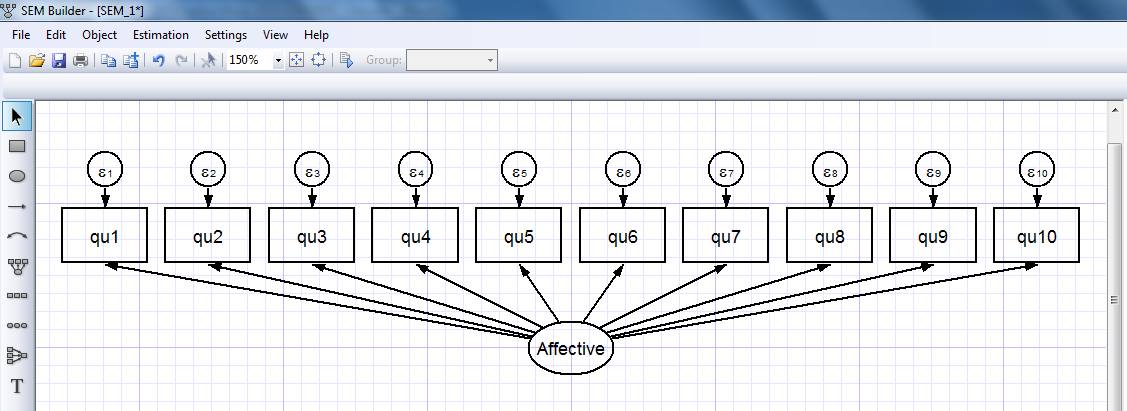
When we click “OK”, the affective measurement component appears in the builder:
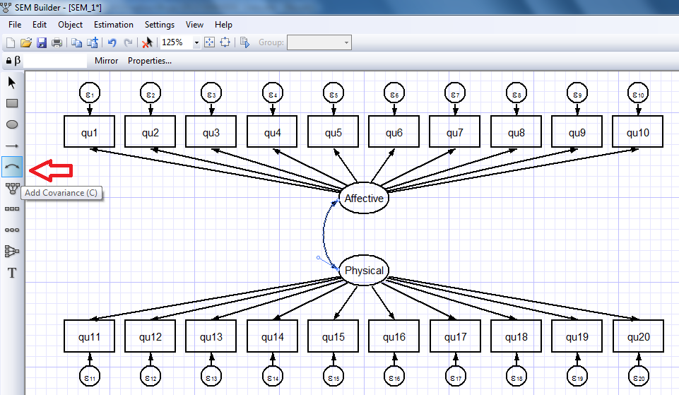
We can repeat this process to create a measurement component for our physical depression scale (images not shown). We can also allow for covariance/correlation between our affective and physical depression scales using the “Add Covariance” icon on the toolbar (red arrow below).
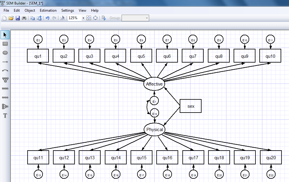
I’ll omit the intermediate steps to build the full model shown below but it’s easy to use the “Add Observed Variable” and “Add Path” icons to create the full model:
Now we’re ready to estimate the parameters for our model. To do this, we click the “Estimate” icon on the toolbar (duh!):
And the flowing dialog box appears:
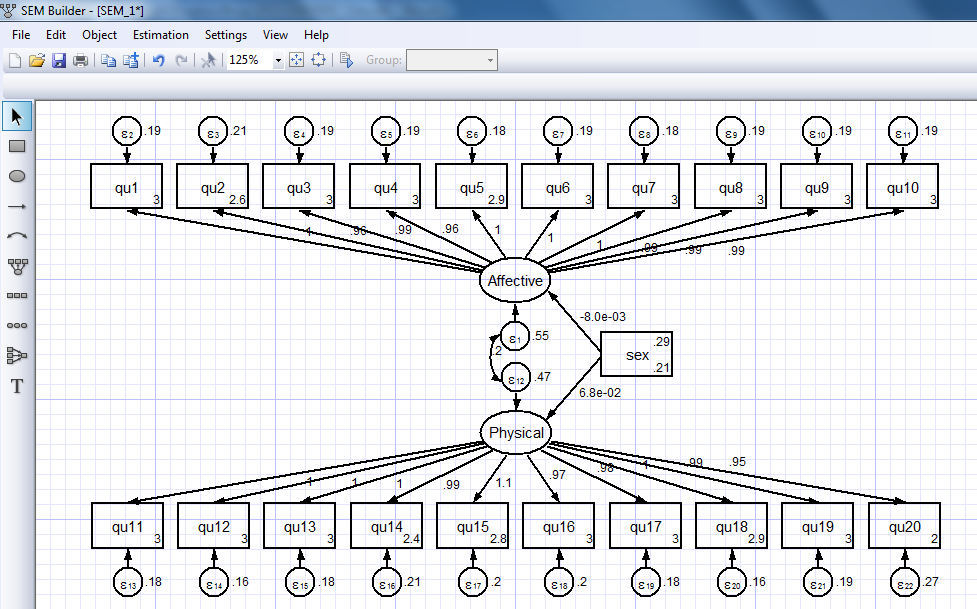
Let’s ignore the estimation options for now and use the default settings. Click “OK” and the parameter estimates will appear in the diagram:
Some of the parameter estimates are difficult to read in this form but it is easy to rearrange the placement and formatting of the estimates to make them easier to read.
If we look at Stata’s output window and scroll up, you’ll notice that the SEM Builder automatically generated the command for our model:
sem (Affective -> qu1) (Affective -> qu2) (Affective -> qu3)
    (Affective -> qu4) (Affective -> qu5) (Affective -> qu6)
    (Affective -> qu7) (Affective -> qu8) (Affective -> qu9)
    (Affective -> qu10) (Physical -> qu11) (Physical -> qu12)
    (Physical -> qu13) (Physical -> qu14) (Physical -> qu15)
    (Physical -> qu16) (Physical -> qu17) (Physical -> qu18)
    (Physical -> qu19) (Physical -> qu20) (sex -> Affective)
    (sex -> Physical), latent(Affective Physical) cov(e.Physical*e.Affective)
We can gather terms and abbreviate some things to make the command much easier to read:
sem (Affective -> qu1-qu10) ///
    (Physical -> qu11-qu20) ///
    (sex -> Affective Physical) ///
    , latent(Affective Physical ) ///
    cov( e.Physical*e.Affective)
We could then calculate a Wald statistic to test the null hypothesis that there is no association between sex and our affective and physical depression scales.
test sex

 ( 1)  [Affective]sex = 0
 ( 2)  [Physical]sex = 0

           chi2(  2) =    2.51
         Prob > chi2 =    0.2854
Final thoughts
This is an admittedly oversimplified example – we haven’t considered the fit of the model or considered any alternative models. We have only included one dichotomous independent variable. We might prefer to use a likelihood ratio test or a score test. Those are all very important issues and should not be ignored in a proper data analysis. But my goal was to demonstrate how easy it is to use Stata’s SEM builder to model data such as those arising from the Beck Depression Inventory. Incidentally, if these data were collected using a complex survey design, it would not be difficult to incorporate the sampling structure and sample weights into the analysis. Missing data can be handled easily as well using Full Information Maximum Likelihood (FIML) but those are topics for another day.
If you would like view the slides from my talk, download the data used in this example or view a video demonstration of Stata’s SEM builder using these data, please use the links below. For the dataset, you can also type use followed by the URL for the data to load it directly into Stata.
Slides:
http://stata.com/meeting/sandiego12/materials/sd12_huber.pdf
Data:
http://stata.com/meeting/sandiego12/materials/Huber_2012SanDiego.dta
YouTube video demonstration:
http://www.youtube.com/watch?v=Xj0gBlqwYHI
References
Beck AT, Ward CH, Mendelson M, Mock J, Erbaugh J (June 1961). An inventory for measuring depression. Arch. Gen. Psychiatry 4 (6): 561–71.
Beck AT, Ward C, Mendelson M (1961). Beck Depression Inventory (BDI). Arch Gen Psychiatry 4 (6): 561–571
Beck AT, Steer RA, Ball R, Ranieri W (December 1996). Comparison of Beck Depression Inventories -IA and -II in psychiatric outpatients. Journal of Personality Assessment 67 (3): 588–97
Bollen, KA. (1989). Structural Equations With Latent Variables. New York, NY: John Wiley and Sons
Kline, RB (2011). Principles and Practice of Structural Equation Modeling. New York, NY: Guilford Press
Raykov, T & Marcoulides, GA (2006). A First Course in Structural Equation Modeling. Mahwah, NJ: Lawrence Erlbaum
Schumacker, RE & Lomax, RG (2012) A Beginner’s Guide to Structural Equation Modeling, 3rd Ed. New York, NY: Routledge
