Understanding the generalized method of moments (GMM): A simple example
\(\newcommand{\Eb}{{\bf E}}\)This post was written jointly with Enrique Pinzon, Senior Econometrician, StataCorp.
The generalized method of moments (GMM) is a method for constructing estimators, analogous to maximum likelihood (ML). GMM uses assumptions about specific moments of the random variables instead of assumptions about the entire distribution, which makes GMM more robust than ML, at the cost of some efficiency. The assumptions are called moment conditions.
GMM generalizes the method of moments (MM) by allowing the number of moment conditions to be greater than the number of parameters. Using these extra moment conditions makes GMM more efficient than MM. When there are more moment conditions than parameters, the estimator is said to be overidentified. GMM can efficiently combine the moment conditions when the estimator is overidentified.
We illustrate these points by estimating the mean of a \(\chi^2(1)\) by MM, ML, a simple GMM estimator, and an efficient GMM estimator. This example builds on Efficiency comparisons by Monte Carlo simulation and is similar in spirit to the example in Wooldridge (2001).
GMM weights and efficiency
GMM builds on the ideas of expected values and sample averages. Moment conditions are expected values that specify the model parameters in terms of the true moments. The sample moment conditions are the sample equivalents to the moment conditions. GMM finds the parameter values that are closest to satisfying the sample moment conditions.
The mean of a \(\chi^2\) random variable with \(d\) degree of freedom is \(d\), and its variance is \(2d\). Two moment conditions for the mean are thus
\[\begin{eqnarray*}
\Eb\left[Y – d \right]&=& 0 \\
\Eb\left[(Y – d )^2 – 2d \right]&=& 0
\end{eqnarray*}\]
The sample moment equivalents are
\[\begin{eqnarray}
1/N\sum_{i=1}^N (y_i – \widehat{d} )&=& 0 \tag{1} \\
1/N\sum_{i=1}^N\left[(y_i – \widehat{d} )^2 – 2\widehat{d}\right] &=& 0 \tag{2}
\end{eqnarray}\]
We could use either sample moment condition (1) or sample moment condition (2) to estimate \(d\). In fact, below we use each one and show that (1) provides a much more efficient estimator.
When we use both (1) and (2), there are two sample moment conditions and only one parameter, so we cannot solve this system of equations. GMM finds the parameters that get as close as possible to solving weighted sample moment conditions.
Uniform weights and optimal weights are two ways of weighting the sample moment conditions. The uniform weights use an identity matrix to weight the moment conditions. The optimal weights use the inverse of the covariance matrix of the moment conditions.
We begin by drawing a sample of a size 500 and use gmm to estimate the parameters using sample moment condition (1), which we illustrate is the sample as the sample average.
. drop _all

. set obs 500
number of observations (_N) was 0, now 500

. set seed 12345

. generate double y = rchi2(1)

. gmm (y - {d})  , instruments( ) onestep

Step 1
Iteration 0:   GMM criterion Q(b) =  .82949186
Iteration 1:   GMM criterion Q(b) =  1.262e-32
Iteration 2:   GMM criterion Q(b) =  9.545e-35

note: model is exactly identified

GMM estimation

Number of parameters =   1
Number of moments    =   1
Initial weight matrix: Unadjusted                 Number of obs   =        500

------------------------------------------------------------------------------
             |               Robust
             |      Coef.   Std. Err.      z    P>|z|     [95% Conf. Interval]
-------------+----------------------------------------------------------------
          /d |   .9107644   .0548098    16.62   0.000     .8033392     1.01819
------------------------------------------------------------------------------
Instruments for equation 1: _cons

. mean y

Mean estimation                   Number of obs   =        500

--------------------------------------------------------------
             |       Mean   Std. Err.     [95% Conf. Interval]
-------------+------------------------------------------------
           y |   .9107644   .0548647      .8029702    1.018559
--------------------------------------------------------------
The sample moment condition is the product of an observation-level error function that is specified inside the parentheses and an instrument, which is a vector of ones in this case. The parameter \(d\) is enclosed in curly braces {}. We specify the onestep option because the number of parameters is the same as the number of moment conditions, which is to say that the estimator is exactly identified. When it is, each sample moment condition can be solved exactly, and there are no efficiency gains in optimally weighting the moment conditions.
We now illustrate that we could use the sample moment condition obtained from the variance to estimate \(d\).
. gmm ((y-{d})^2 - 2*{d})  , instruments( ) onestep

Step 1
Iteration 0:   GMM criterion Q(b) =  5.4361161
Iteration 1:   GMM criterion Q(b) =  .02909692
Iteration 2:   GMM criterion Q(b) =  .00004009
Iteration 3:   GMM criterion Q(b) =  5.714e-11
Iteration 4:   GMM criterion Q(b) =  1.172e-22

note: model is exactly identified

GMM estimation

Number of parameters =   1
Number of moments    =   1
Initial weight matrix: Unadjusted                 Number of obs   =        500

------------------------------------------------------------------------------
             |               Robust
             |      Coef.   Std. Err.      z    P>|z|     [95% Conf. Interval]
-------------+----------------------------------------------------------------
          /d |   .7620814   .1156756     6.59   0.000     .5353613    .9888015
------------------------------------------------------------------------------
Instruments for equation 1: _cons
While we cannot say anything definitive from only one draw, we note that this estimate is further from the truth and that the standard error is much larger than those based on the sample average.
Now, we use gmm to estimate the parameters using uniform weights.
. matrix I = I(2)

. gmm ( y - {d}) ( (y-{d})^2 - 2*{d})  , instruments( ) winitial(I) onestep

Step 1
Iteration 0:   GMM criterion Q(b) =   6.265608
Iteration 1:   GMM criterion Q(b) =  .05343812
Iteration 2:   GMM criterion Q(b) =  .01852592
Iteration 3:   GMM criterion Q(b) =   .0185221
Iteration 4:   GMM criterion Q(b) =   .0185221

GMM estimation

Number of parameters =   1
Number of moments    =   2
Initial weight matrix: user                       Number of obs   =        500

------------------------------------------------------------------------------
             |               Robust
             |      Coef.   Std. Err.      z    P>|z|     [95% Conf. Interval]
-------------+----------------------------------------------------------------
          /d |   .7864099   .1050692     7.48   0.000     .5804781    .9923418
------------------------------------------------------------------------------
Instruments for equation 1: _cons
Instruments for equation 2: _cons
The first set of parentheses specifies the first sample moment condition, and the second set of parentheses specifies the second sample moment condition. The options winitial(I) and onestep specify uniform weights.
Finally, we use gmm to estimate the parameters using two-step optimal weights. The weights are calculated using first-step consistent estimates.
. gmm ( y - {d}) ( (y-{d})^2 - 2*{d})  , instruments( ) winitial(I)

Step 1
Iteration 0:   GMM criterion Q(b) =   6.265608
Iteration 1:   GMM criterion Q(b) =  .05343812
Iteration 2:   GMM criterion Q(b) =  .01852592
Iteration 3:   GMM criterion Q(b) =   .0185221
Iteration 4:   GMM criterion Q(b) =   .0185221

Step 2
Iteration 0:   GMM criterion Q(b) =  .02888076
Iteration 1:   GMM criterion Q(b) =  .00547223
Iteration 2:   GMM criterion Q(b) =  .00546176
Iteration 3:   GMM criterion Q(b) =  .00546175

GMM estimation

Number of parameters =   1
Number of moments    =   2
Initial weight matrix: user                       Number of obs   =        500
GMM weight matrix:     Robust

------------------------------------------------------------------------------
             |               Robust
             |      Coef.   Std. Err.      z    P>|z|     [95% Conf. Interval]
-------------+----------------------------------------------------------------
          /d |   .9566219   .0493218    19.40   0.000     .8599529    1.053291
------------------------------------------------------------------------------
Instruments for equation 1: _cons
Instruments for equation 2: _cons
All four estimators are consistent. Below we run a Monte Carlo simulation to see their relative efficiencies. We are most interested in the efficiency gains afforded by optimal GMM. We include the sample average, the sample variance, and the ML estimator discussed in Efficiency comparisons by Monte Carlo simulation. Theory tells us that the optimally weighted GMM estimator should be more efficient than the sample average but less efficient than the ML estimator.
The code below for the Monte Carlo builds on Efficiency comparisons by Monte Carlo simulation, Maximum likelihood estimation by mlexp: A chi-squared example, and Monte Carlo simulations using Stata. Click gmmchi2sim.do to download this code.
. clear all
. set seed 12345
. matrix I = I(2)
. postfile sim  d_a d_v d_ml d_gmm d_gmme using efcomp, replace
. forvalues i = 1/2000 {
  2.     quietly drop _all
  3.     quietly set obs 500
  4.     quietly generate double y = rchi2(1)
  5.
.     quietly mean y
  6.     local d_a         =  _b[y]
  7.
.     quietly gmm ( (y-{d=`d_a'})^2 - 2*{d}) , instruments( )  ///
>       winitial(unadjusted) onestep conv_maxiter(200)
  8.     if e(converged)==1 {
  9.             local d_v = _b[d:_cons]
 10.     }
 11.     else {
 12.             local d_v = .
 13.     }
 14.
.     quietly mlexp (ln(chi2den({d=`d_a'},y)))
 15.     if e(converged)==1 {
 16.             local d_ml  =  _b[d:_cons]
 17.     }
 18.     else {
 19.             local d_ml  = .
 20.     }
 21.
.     quietly gmm ( y - {d=`d_a'}) ( (y-{d})^2 - 2*{d}) , instruments( )  ///
>         winitial(I) onestep conv_maxiter(200)
 22.     if e(converged)==1 {
 23.             local d_gmm = _b[d:_cons]
 24.     }
 25.     else {
 26.             local d_gmm = .
 27.     }
 28.
.     quietly gmm ( y - {d=`d_a'}) ( (y-{d})^2 - 2*{d}) , instruments( )  ///
>        winitial(unadjusted, independent) conv_maxiter(200)
 29.     if e(converged)==1 {
 30.             local d_gmme = _b[d:_cons]
 31.     }
 32.     else {
 33.             local d_gmme = .
 34.     }
 35.
.     post sim (`d_a') (`d_v') (`d_ml') (`d_gmm') (`d_gmme')
 36.
. }
. postclose sim
. use efcomp, clear
. summarize

    Variable |        Obs        Mean    Std. Dev.       Min        Max
-------------+---------------------------------------------------------
         d_a |      2,000     1.00017    .0625367   .7792076    1.22256
         d_v |      1,996    1.003621    .1732559   .5623049   2.281469
        d_ml |      2,000    1.002876    .0395273   .8701175   1.120148
       d_gmm |      2,000    .9984172    .1415176   .5947328   1.589704
      d_gmme |      2,000    1.006765    .0540633   .8224731   1.188156
The simulation results indicate that the ML estimator is the most efficient (d_ml, std. dev. 0.0395), followed by the efficient GMM estimator (d_gmme}, std. dev. 0.0541), followed by the sample average (d_a, std. dev. 0.0625), followed by the uniformly-weighted GMM estimator (d_gmm, std. dev. 0.1415), and finally followed by the sample-variance moment condition (d_v, std. dev. 0.1732).
The estimator based on the sample-variance moment condition does not converge for 4 of 2,000 draws; this is why there are only 1,996 observations on d_v when there are 2,000 observations for the other estimators. These convergence failures occurred even though we used the sample average as the starting value of the nonlinear solver.
For a better idea about the distributions of these estimators, we graph the densities of their estimates.
Figure 1: Densities of the estimators
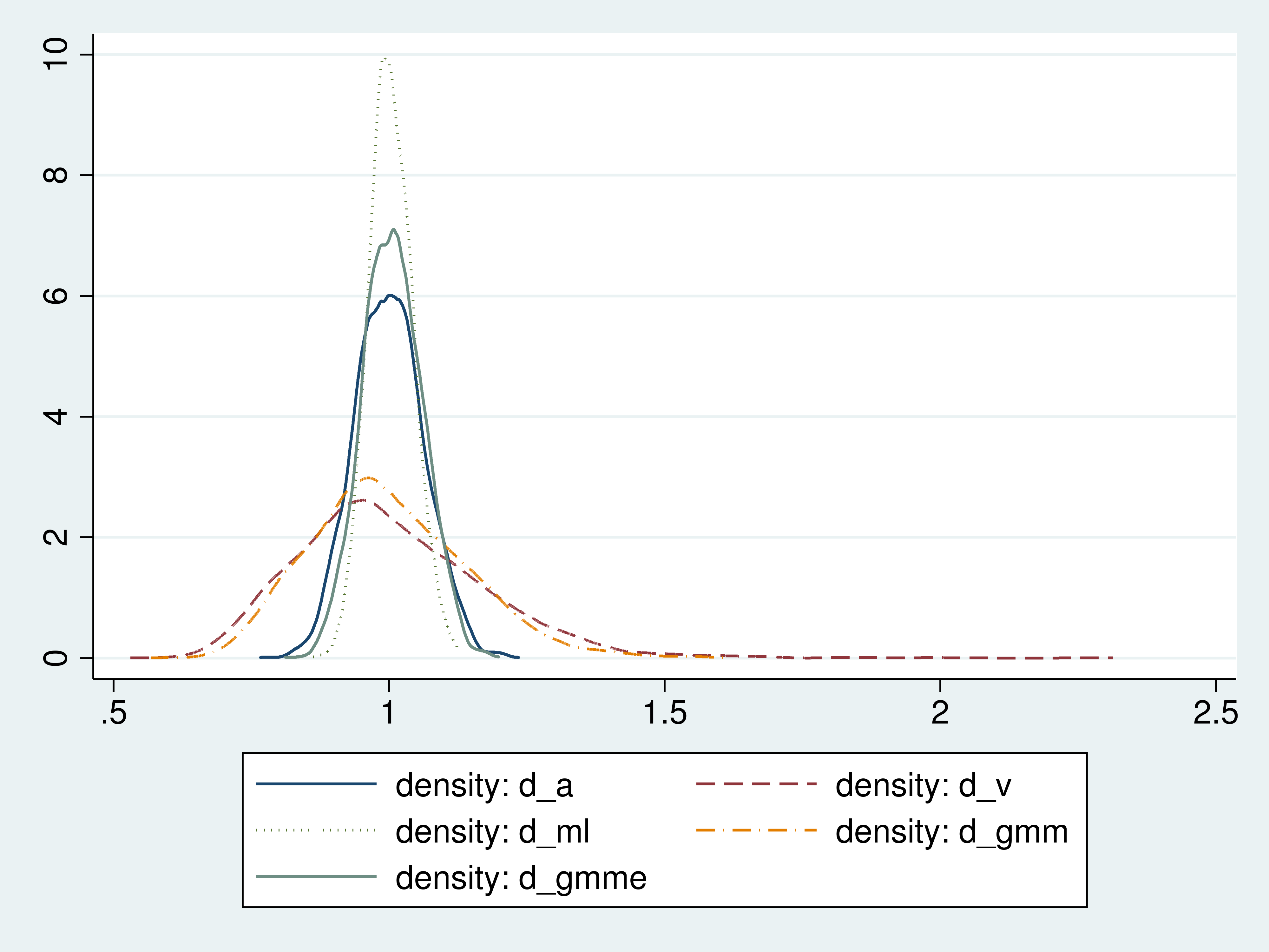
The density plots illustrate the efficiency ranking that we found from the standard deviations of the estimates.
The uniformly weighted GMM estimator is less efficient than the sample average because it places the same weight on the sample average as on the much less efficient estimator based on the sample variance.
In each of the overidentified cases, the GMM estimator uses a weighted average of two sample moment conditions to estimate the mean. The first sample moment condition is the sample average. The second moment condition is the sample variance. As the Monte Carlo results showed, the sample variance provides a much less efficient estimator for the mean than the sample average.
The GMM estimator that places equal weights on the efficient and the inefficient estimator is much less efficient than a GMM estimator that places much less weight on the less efficient estimator.
We display the weight matrix from our optimal GMM estimator to see how the sample moments were weighted.
. quietly gmm ( y - {d}) ( (y-{d})^2 - 2*{d})  , instruments( ) winitial(I)

. matlist e(W), border(rows)

-------------------------------------
             | 1         | 2
             |     _cons |     _cons
-------------+-----------+-----------
1            |           |
       _cons |  1.621476 |
-------------+-----------+-----------
2            |           |
       _cons | -.2610053 |  .0707775
-------------------------------------
The diagonal elements show that the sample-mean moment condition receives more weight than the less efficient sample-variance moment condition.
Done and undone
We used a simple example to illustrate how GMM exploits having more equations than parameters to obtain a more efficient estimator. We also illustrated that optimally weighting the different moments provides important efficiency gains over an estimator that uniformly weights the moment conditions.
Our cursory introduction to GMM is best supplemented with a more formal treatment like the one in Cameron and Trivedi (2005) or Wooldridge (2010).
Graph code appendix
use efcomp
local N = _N
kdensity d_a,     n(`N') generate(x_a    den_a)    nograph
kdensity d_v,     n(`N') generate(x_v    den_v)    nograph
kdensity d_ml,    n(`N') generate(x_ml   den_ml)   nograph
kdensity d_gmm,   n(`N') generate(x_gmm  den_gmm)  nograph
kdensity d_gmme,  n(`N') generate(x_gmme den_gmme) nograph
twoway (line den_a x_a,       lpattern(solid))        ///
       (line den_v x_v,       lpattern(dash))         ///
       (line den_ml x_ml,     lpattern(dot))          ///
       (line den_gmm x_gmm,   lpattern(dash_dot))     ///
       (line den_gmme x_gmme, lpattern(shordash))
References
Cameron, A. C., and P. K. Trivedi. 2005. Microeconometrics: Methods and applications. Cambridge: Cambridge University Press.
Wooldridge, J. M. 2001. Applications of generalized method of moments estimation. Journal of Economic Perspectives 15(4): 87-100.
Wooldridge, J. M. 2010. Econometric Analysis of Cross Section and Panel Data. 2nd ed. Cambridge, Massachusetts: MIT Press.