probit or logit: ladies and gentlemen, pick your weapon
We often use probit and logit models to analyze binary outcomes. A case can be made that the logit model is easier to interpret than the probit model, but Stata’s margins command makes any estimator easy to interpret. Ultimately, estimates from both models produce similar results, and using one or the other is a matter of habit or preference.
I show that the estimates from a probit and logit model are similar for the computation of a set of effects that are of interest to researchers. I focus on the effects of changes in the covariates on the probability of a positive outcome for continuous and discrete covariates. I evaluate these effects on average and at the mean value of the covariates. In other words, I study the average marginal effects (AME), the average treatment effects (ATE), the marginal effects at the mean values of the covariates (MEM), and the treatment effects at the mean values of the covariates (TEM).
First, I present the results. Second, I discuss the code used for the simulations.
Results
In Table 1, I present the results of a simulation with 4,000 replications when the true data generating process (DGP) satisfies the assumptions of a probit model. I show the average of the AME and the ATE estimates and the 5% rejection rate of the true null hypothesis that arise after probit and logit estimation. I also provide an approximate true value of the AME and ATE. I obtain the approximate true values by computing the ATE and AME, at the true values of the coefficients, using a sample of 20 million observations. I will provide more details on the simulation in a later section.
Table 1: Average Marginal and Treatment Effects: True DGP Probit
| Statistic | Approximate True Value | Probit | Logit |
|---|---|---|---|
| AME of x1 | -.1536 | -.1537 | -.1537 |
| 5% Rejection Rate | .050 | .052 | |
| ATE of x2 | .1418 | .1417 | .1417 |
| 5% Rejection Rate | .050 | .049 |
For the MEM and TEM, we have the following:
Table 2: Marginal and Treatment Effects at Mean Values: True DGP Probit
| Statistic | Approximate True Value | Probit | Logit |
|---|---|---|---|
| MEM of x1 | -.1672 | -.1673 | -.1665 |
| 5% Rejection Rate | .056 | .06 | |
| TEM of x2 | .1499 | .1498 | .1471 |
| 5% Rejection Rate | .053 | .058 |
The logit estimates are close to the true value and have a rejection rate that is close to 5%. Fitting the parameters of our model using logit when the true DGP satisfies the assumptions of a probit model does not lead us astray.
If the true DGP satisfies the assumptions of the logit model, the conclusions are the same. I present the results in the next two tables.
Table 3: Average Marginal and Treatment Effects: True DGP Logit
| Statistic | Approximate True Value | Probit | Logit |
|---|---|---|---|
| AME of x1 | -.1090 | -.1088 | -.1089 |
| 5% Rejection Rate | .052 | .052 | |
| ATE of x2 | .1046 | .1044 | .1045 |
| 5% Rejection Rate | .053 | .051 |
Table 4: Marginal and Treatment Effects at Mean Values: True DGP Logit
| Statistic | Approximate True Value | Probit | Logit |
|---|---|---|---|
| MEM of x1 | -.1146 | -.1138 | -.1146 |
| 5% Rejection Rate | .050 | .051 | |
| TEM of x2 | .1086 | .1081 | .1085 |
| 5% Rejection Rate | .058 | .058 |
Why?
Maximum likelihood estimators find the parameters that maximize the likelihood that our data will fit the distributional assumptions that we make. The likelihood chosen is an approximation to the true likelihood, and it is a helpful approximation if the true likelihood and our approximating are close to each other. Viewing likelihood-based models as useful approximations, instead of as models of a true likelihood, is the basis of quasilikelihood theory. For more details, see White (1996) and Wooldridge (2010).
It is assumed that the unobservable random variable in the probit model and logit model comes from a standard normal and logistic distribution, respectively. The cumulative distribution functions (CDFs) in these two cases are close to each other, especially around the mean. Therefore, estimators under these two sets of assumptions produce similar results. To illustrate these arguments, we can plot the two CDFs and their differences as follows:
Graph 1: Normal and Logistic CDF’s and their Difference
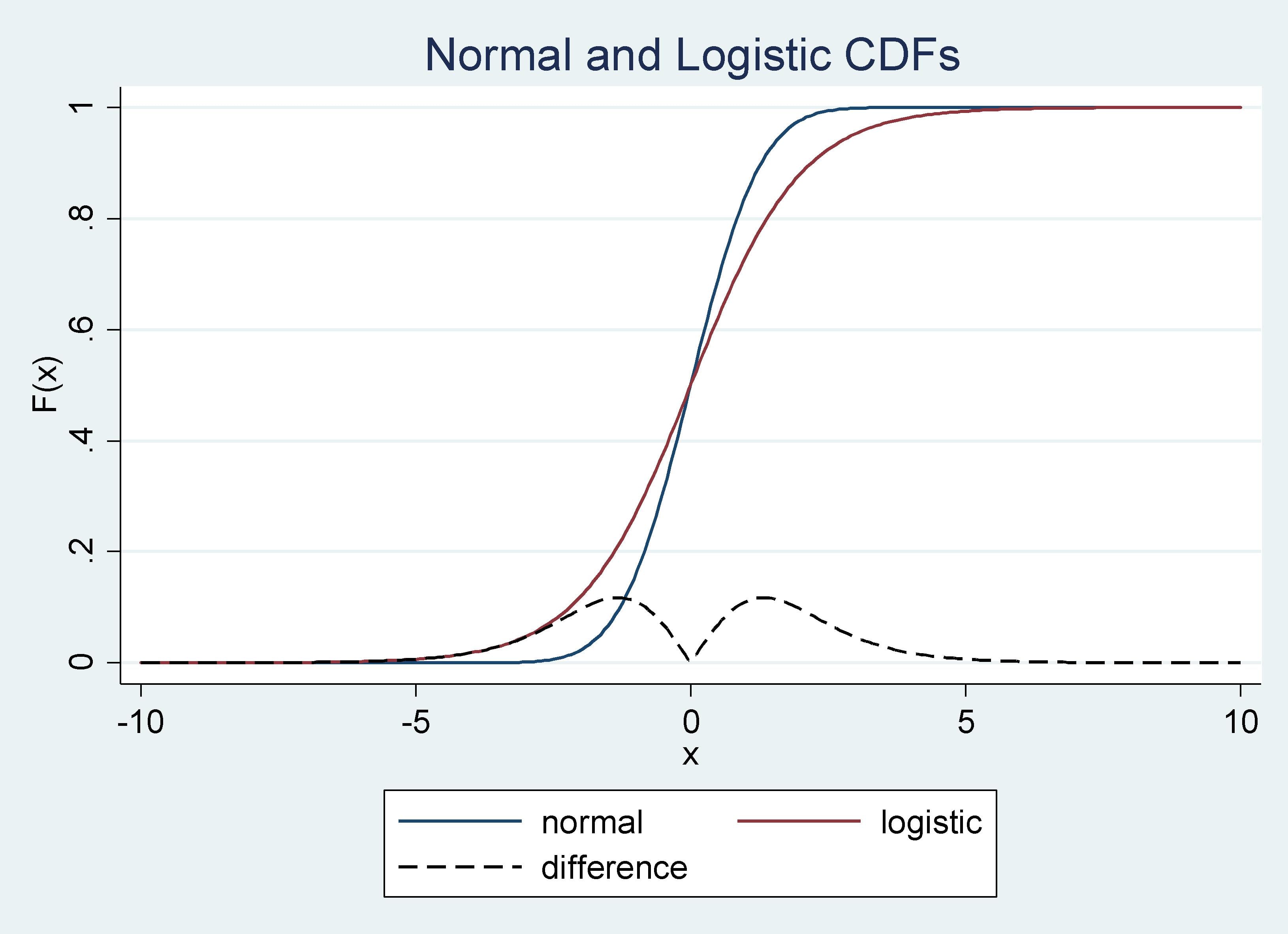
The difference between the CDFs approaches zero as you get closer to the mean, from the right or from the left, and it is always smaller than .15.
Simulation design
Below is the code I used to generate the data for my simulations. In the first part, lines 4 to 12, I generate outcome variables that satisfy the assumptions of the probit model, y1, and the logit model, y2. In the second part, lines 13 to 16, I compute the marginal effects for the logit and probit models. I have a continuous and a discrete covariate. For the discrete covariate, the marginal effect is a treatment effect. In the third part, lines 17 to 25, I compute the marginal effects evaluated at the means. I will use these estimates later to compute approximations to the true values of the effects.
program define mkdata
        syntax, [n(integer 1000)]
        clear
        quietly set obs `n'
        // 1. Generating data from probit, logit, and misspecified
        generate x1    = rnormal()
        generate x2    = rbeta(2,4)>.5
        generate e1    = rnormal()
        generate u     = runiform()
        generate e2    = ln(u) -ln(1-u)
        generate xb    = .5*(1 -x1 + x2)
        generate y1    =  xb + e1 > 0
        generate y2    =  xb + e2 > 0
        // 2. Computing probit & logit marginal and treatment effects
        generate m1    = normalden(xb)*(-.5)
        generate m2    = normal(1 -.5*x1 ) - normal(.5 -.5*x1)
        generate m1l   = exp(xb)*(-.5)/(1+exp(xb))^2
        generate m2l   = exp(1 -.5*x1)/(1+ exp(1 -.5*x1 )) - ///
                         exp(.5 -.5*x1)/(1+ exp(.5 -.5*x1 ))
        // 3. Computing probit & logit marginal and treatment effects at means
        quietly mean x1 x2
        matrix A         = r(table)
        scalar a         = .5 -.5*A[1,1] + .5*A[1,2]
        scalar b1        =  1 -.5*A[1,1]
        scalar b0        = .5 -.5*A[1,1]
        generate mean1   = normalden(a)*(-.5)
        generate mean2   = normal(b1) - normal(b0)
        generate mean1l  = exp(a)*(-.5)/(1+exp(a))^2
        generate mean2l  = exp(b1)/(1+ exp(b1)) - exp(b0)/(1+ exp(b0))
end
I approximate the true marginal effects using a sample of 20 million observations. This is a reasonable strategy in this case. For example, take the average marginal effect for a continuous covariate, \(x_{k}\), in the case of the probit model:
\[\begin{equation*}
\frac{1}{N}\sum_{i=1}^N \phi\left(x_{i}\mathbb{\beta}\right)\beta_{k}
\end{equation*}\]
The expression above is an approximation to \(E\left(\phi\left(x_{i}\mathbb{\beta}\right)\beta_{k}\right)\). To obtain this expected value, we would need to integrate over the distribution of all the covariates. This is not practical and would limit my choice of covariates. Instead, I draw a sample of 20 million observations, compute \(\frac{1}{N}\sum_{i=1}^N \phi\left(x_{i}\mathbb{\beta}\right)\beta_{k}\), and take it to be the true value. I follow the same logic for the other marginal effects.
Below is the code I use to compute the approximate true marginal effects. I draw the 20 million observations, then I compute the averages that I am going to use in my simulation, and I create locals for each approximate true value.
. mkdata, n(20000000)

. local values "m1 m2 m1l m2l mean1 mean2 mean1l mean2l"

. local means  "mx1 mx2 mx1l mx2l meanx1 meanx2 meanx1l meanx2l"

. local n : word count `values'

. forvalues i= 1/`n' {
  2.         local a: word `i' of `values'
  3.         local b: word `i' of `means'
  4.         sum `a', meanonly
  5.         local `b' = r(mean)
  6. }
Now I am ready to run all the simulations that I used to produce the results in the previous section. The code that I used for the simulations for the ATE and the AME when the true DGP is a probit is given by
. postfile mprobit y1p y1p_r y1l y1l_r y2p y2p_r y2l y2l_r ///
>                 using simsmprobit, replace

. forvalues i=1/4000 {
  2.         quietly {
  3.                 mkdata, n(10000)
  4.                 probit y1 x1 i.x2, vce(robust)
  5.                 margins, dydx(*) atmeans post
  6.                 local y1p = _b[x1]
  7.                 test _b[x1] = `meanx1'
  8.                 local y1p_r   = (r(p)<.05)
  9.                 local y2p = _b[1.x2]
 10.                 test _b[1.x2] = `meanx2'
 11.                 local y2p_r   = (r(p)<.05)
 12.                 logit  y1 x1 i.x2, vce(robust)
 13.                 margins, dydx(*) atmeans post
 14.                 local y1l = _b[x1]
 15.                 test _b[x1] = `meanx1'
 16.                 local y1l_r   = (r(p)<.05)
 17.                 local y2l = _b[1.x2]
 18.                 test _b[1.x2] = `meanx2'
 19.                 local y2l_r   = (r(p)<.05)
 20.                 post mprobit (`y1p') (`y1p_r') (`y1l') (`y1l_r') ///
>                            (`y2p') (`y2p_r') (`y2l') (`y2l_r')
 21.         }
 22. }
. use simsprobit
. summarize

    Variable |        Obs        Mean    Std. Dev.       Min        Max
-------------+---------------------------------------------------------
         y1p |      4,000   -.1536812    .0038952  -.1697037  -.1396532
       y1p_r |      4,000         .05    .2179722          0          1
         y1l |      4,000   -.1536778    .0039179  -.1692524  -.1396366
       y1l_r |      4,000      .05175    .2215496          0          1
         y2p |      4,000     .141708    .0097155   .1111133   .1800973
-------------+---------------------------------------------------------
       y2p_r |      4,000       .0495    .2169367          0          1
         y2l |      4,000    .1416983    .0097459   .1102069   .1789895
       y2l_r |      4,000        .049     .215895          0          1
For the results in the case of the MEM and the TEM when the true DGP is a probit, I use margins with the option atmeans. The other cases are similar. I use robust standard error for all computations to account for the fact that my likelihood model is an approximation to the true likelihood, and I use the option vce(unconditional) to account for the fact that I am using two-step M-estimation. See Wooldridge (2010) for more details on two-step M-estimation.
You can download the code used to produce the results by clicking this link: pvsl.do
Concluding remarks
I provided simulation evidence that illustrates that the differences between using estimates of effects after probit or logit is negligible. The reason lies in the theory of quasilikelihood and, specifically, in that the cumulative distribution functions of the probit and logit models are similar, especially around the mean.
References
White, H. 1996. Estimation, Inference, and Specification Analysis>. Cambridge: Cambridge University Press.
Wooldridge, J. M. 2010. Econometric Analysis of Cross Section and Panel Data. 2nd ed. Cambridge, Massachusetts: MIT Press.