\(\newcommand{\mub}{{\boldsymbol{\mu}}}
\newcommand{\eb}{{\boldsymbol{e}}}
\newcommand{\betab}{\boldsymbol{\beta}}\)Applied time-series researchers often want to compare the accuracy of a pair of competing forecasts. A popular statistic for forecast comparison is the mean squared forecast error (MSFE), a smaller value of which implies a better forecast. However, a formal test, such as Diebold and Mariano (1995), distinguishes whether the superiority of one forecast is statistically significant or is simply due to sampling variability.

A related test is the forecast encompassing test. This test is used to determine whether one of the forecasts encompasses all the relevant information from the other. The resulting test statistic may lead a researcher to either combine the two forecasts or drop the forecast that contains no additional information.

In this post, I construct a pair of one-step-ahead recursive forecasts for the change in inflation rate from an autoregression model (AR) and a vector autoregression model (VAR). Based on an exercise in Clark and McCracken (2001), I consider a bivariate VAR with changes in inflation and unemployment rate as dependent variables. I compare the forecasts using MSFE, perform tests of predictive accuracy and forecast encompassing to determine whether unemployment rate is useful in predicting inflation rate. Because the VAR model nests the AR model, I assess the significance of the test statistic using appropriate critical values provided in McCracken (2007) and Clark and McCracken (2001).

Forecasting methods

Let \(y_t\) denote a series we want to forecast and \(\hat{y}_{t+h|t}\) denote the \(h\)-step-ahead forecast of \(y_t\) at time \(t\). Out-of-sample forecasts are usually computed with a fixed, rolling, or recursive window method. In all the methods, an initial sample of \(T\) observations is used to estimate the parameters of the model. In a fixed window method, estimation is performed once in a sample of \(T\) observations and \(h\)-step-ahead forecasts are made based on those estimates. In a rolling window method, the size of the estimation sample is kept fixed. However, estimation is performed multiple times by incrementing the beginning and end of the initial sample by the same number. Out-of-sample forecasts are computed after each estimation. A recursive window method is similar to a rolling window method except that the beginning time period is held fixed while the the ending period increases.

I use the rolling prefix command with the recursive option to generate recursive forecasts. rolling executes the command it prefixes on a window of observations and stores results such as parameter estimates or other summary statistics. In the following section, I write commands that fit AR(2) and VAR(2) models, compute one-step-ahead forecasts, and return relevant statistics. I use these commands with the rolling prefix and store the recursive forecasts in a new dataset.

Programming a command for the rolling prefix

In usinfl.dta, I have quarterly data from 1948q1 to 2016q1 on the changes in inflation rate and the unemployment rate obtained from the St. Louis FRED database. The first model is an AR(2) model of change in inflation, which is given by
\[
{\tt dinflation}_{\,\,t} = \beta_0 + \beta_1 {\tt dinflation}_{\,\,t-1} +
\beta_2 {\tt dinflation}_{\,\,t-2} + \epsilon_t
\]
where \(\beta_0\) is the intercept and \(\beta_1\) and \(\beta_2\) are the AR parameters. I generate recursive forecasts for these models beginning in 2002q2. This implies an initial window size of 218 observations from 1948q1 to 2002q1. The choice of the window size for computing forecasts in applied research is arbitrary. See Rossi and Inoue (2012) for tests of predictive accuracy that is robust to the choice of window size.

In the following code block, I have a command labeled fcst_ar2.ado that estimates the parameters of an AR(2) model using regress and computes one-step-ahead forecasts.

program fcst_ar2, rclass
        syntax [if]

        qui tsset
        local timevar `r(timevar)'
        local first `r(tmin)'

        regress l(0/2).dinflation `if'
        summarize `timevar' if e(sample)

        local last = `r(max)'-`first'+1
        local fcast = _b[_cons] + _b[l.dinflation]*     ///
                dinflation[`last'] + _b[l2.dinflation]* ///
                dinflation[`last'-1]

        return scalar fcast = `fcast'
        return scalar actual = dinflation[`last'+1]
        return scalar sqerror = (dinflation[`last'+1]-  ///
                `fcast')^2
end

Line 1 defines the name of the command and declares it to be rclass so that I can return my results in r() after executing the command. Line 2 defines the syntax for the command. I specify an if qualifier in the syntax so that my command can identify the correct observations when used with the rolling prefix. Lines 4–6 store the time variable and the beginning time index in my dataset as local macros timevar and first, respectively. Lines 8–9 use regress to fit an AR(2) model and summarize the time variable in the sample used for estimation. Line 11 stores the last time index in the local macro last. The one-step-ahead forecast for the AR(2) model is
\[
\hat{y}_{t+1|t} = \hat{\beta}_0 + \hat{\beta}_1 {\tt dinflation}_{\,\,t-1} + \hat{\beta}_2 {\tt dinflation}_{\,\,t-2}
\]
where \(\hat{\beta}\)’s are the estimated parameters. Lines 12–14 store the forecast in a local macro fcast. Lines 16–19 return the forecasted value, actual value, and the squared error in local macros fcast, actual, and sqerror, respectively. Line 20 specifies the end of the command.

The second model is a VAR(2) model of change in inflation and unemployment rate and is given by
\[
\begin{bmatrix} {\tt dinflation}_{\,\,t} \\
{\tt dunrate}_{\,\,t}
\end{bmatrix}
= \mub + {\bf B}_1 \begin{bmatrix} {\tt
dinflation}_{\,\,t-1}\\ {\tt dunrate}_{\,\,t-1}
\end{bmatrix}
+ {\bf B}_2 \begin{bmatrix}
{\tt dinflation}_{\,\,t-2}\\
{\tt dunrate}_{\,\,t-2}
\end{bmatrix} + \eb_t
\]
where \(\mub\) is a \(2\times 1\) vector of intercepts, \({\bf B}_1\) and \({\bf B}_2\) are \(2\times 2\) matrices of parameters, and \(\eb_t\) is a \(2\times 1\) vector of IID errors with mean \({\bf 0}\) and covariance \(\boldsymbol{\Sigma}\).

In the following code block, I have a command called fcst_var2.ado that estimates the parameters of a VAR(2) model using var and computes one-step-ahead forecasts.

program fcst_var2, rclass

        syntax [if]

        quietly tsset
        local timevar `r(timevar)'
        local first `r(tmin)'

        var dinflation dunrate `if'
        summarize `timevar' if e(sample)

        local last = `r(max)'-`first'+1
        local fcast = _b[dinflation:_cons] +             ///
                _b[dinflation:l.dinflation]*             ///
                dinflation[`last'] +                     ///
                _b[dinflation:l2.dinflation]*            ///
                dinflation[`last'-1] +                   ///
                _b[dinflation:l.dunrate]*dunrate[`last'] ///
                + _b[dinflation:l2.dunrate]*dunrate[`last'-1]

        return scalar fcast = `fcast'
        return scalar actual = dinflation[`last'+1]
        return scalar sqerror = (dinflation[`last'+1]-   ///
                `fcast')^2
end

The structure of this command is similar to the AR(2) I described earlier. The one-step-ahead forecast of dinflation equation for the VAR(2) model is
\[
\hat{y}_{t+1|t} = \hat{\mu}_1 + \hat{\beta}_{1,11} {\tt
dinflation}_{\,\,t-1} + \hat{\beta}_{1,12} {\tt dunrate}_{\,\,t-1} +
\hat{\beta}_{2,11} {\tt dinflation}_{\,\,t-2} \\
+ \hat{\beta}_{2,12}
{\tt dunrate}_{\,\,t-2}
\]
where \(\hat{\mu}_1\) and \(\hat{\beta}\)’s are the estimated parameters corresponding to the dinflation equation. Lines 13–19 store the one-step-ahead forecast in local macro fcast.

Recursive forecasts

I use the rolling prefix command with the command fcst_ar2. The squared errors, one-step-ahead forecast, and the actual values returned by fcst_ar2 are stored in variables named ar2_sqerror, ar2_fcst, and actual, respectively. I specify a window size of 218 and store the estimates in the dataset ar2.

. use usinfl, clear

. rolling ar2_sqerr=r(sqerror) ar2_fcast=r(fcast) actual=r(actual), 
> window(218) recursive saving(ar2, replace): fcst_ar2
(running fcst_ar2 on estimation sample)

Rolling replications (56)
----+--- 1 ---+--- 2 ---+--- 3 ---+--- 4 ---+--- 5
..................................................    50
.....e
file ar2.dta saved

With a window size of 218, I have 55 usable observations that are one-step-ahead forecasts. I do the same with fcst_var2 below and store the estimates in the dataset var2.

. rolling var2_sqerr=r(sqerror) var2_fcast=r(fcast), window(218) 
> recursive saving(var2, replace): fcst_var2
(running fcst_var2 on estimation sample)

Rolling replications (56)
----+--- 1 ---+--- 2 ---+--- 3 ---+--- 4 ---+--- 5
..................................................    50
.....e
file var2.dta saved

I merge the two datasets containing the forecasts and label the actual and forecast variables. I plot the actual versus the forecasts of dinflation obtained from an AR(2) and a VAR(2) model respectively.

. use ar2, clear
(rolling: fcst_ar2)

. quietly merge 1:1 end using var2

. tsset end
        time variable:  end, 2002q2 to 2016q1
                delta:  1 quarter

. label var end "Quarterly date"

. label var actual "Change in inflation"

. label var ar2_fcast "Forecasts from AR(2)"

. label var var2_fcast "Forecasts from VAR(2)"

. tsline actual ar2_fcast var2_fcast, title("Actual vs Forecasts")

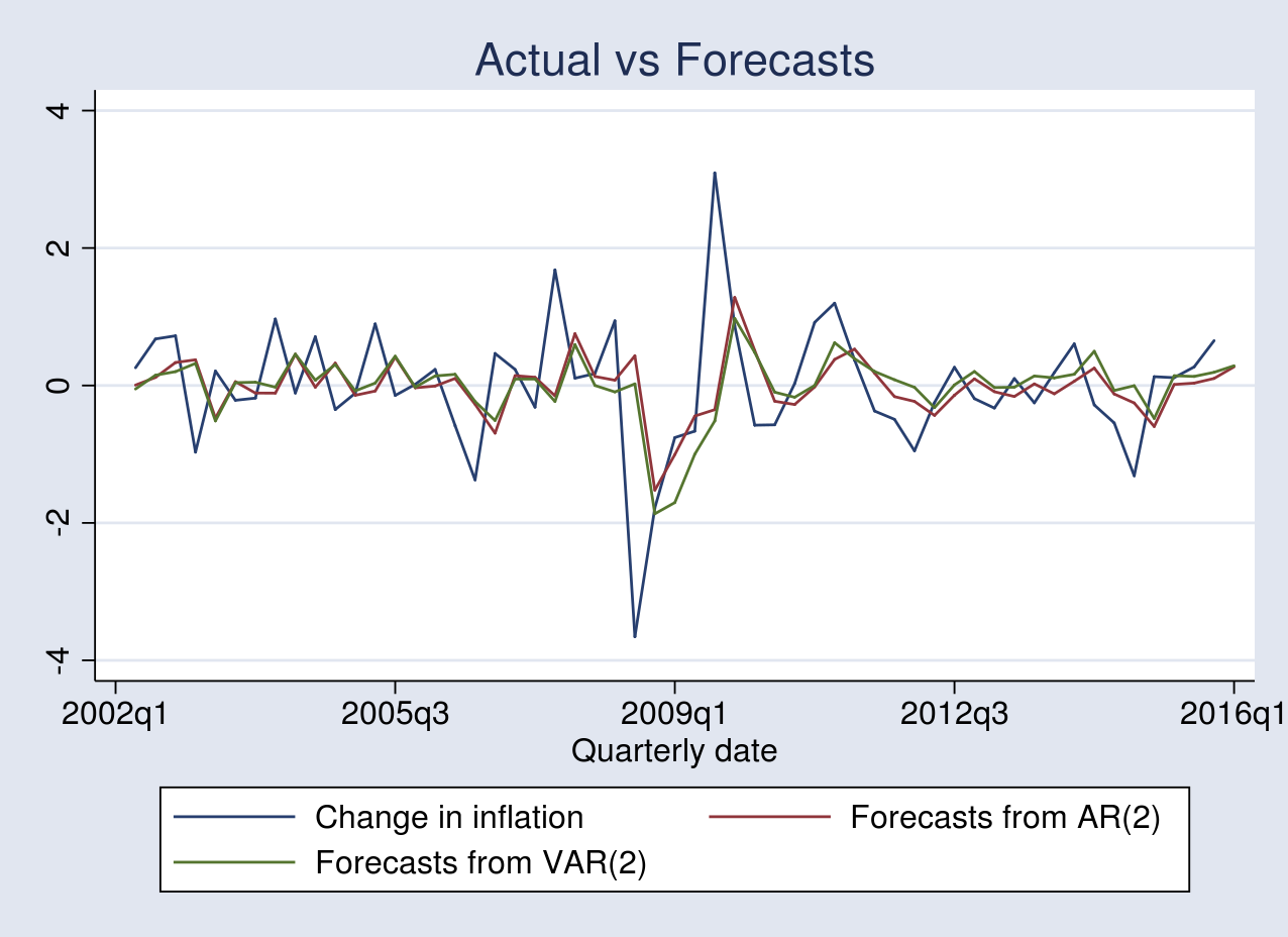
Both models produce forecasts that track the actual change in inflation. However, the performance of one forecast from the other is indistinguishable from the figure above.

Comparing MSFE

A popular statistic used to compare out-of-sample forecasts is the MSFE. I use the mean command to compute this.

. mean ar2_sqerr var2_sqerr

Mean estimation                   Number of obs   =         55

--------------------------------------------------------------
             |       Mean   Std. Err.     [95% Conf. Interval]
-------------+------------------------------------------------
   ar2_sqerr |   .9210348   .3674181      .1844059    1.657664
  var2_sqerr |   .9040102   .3377726      .2268169    1.581203
--------------------------------------------------------------

The MSFE of the forecasts produced by the VAR(2) model is slightly smaller than that of the AR(2) model. This comparison, however, is based on a single sample and does not reflect the predictive performance in the population.

Test for equal predictive accuracy

McCracken (2007) provides test statistics to test the predictive accuracy of forecasts generated by a pair of nested parametric models. Under the null hypothesis, the expected loss of the pair of forecasts is the same. Under the alternative, the expected loss of the bigger model is less than that of the one it nests. In the current application, the null and the alternative hypothesis are as follows
\[
H_o: E[L_{t+1}(\betab_1)] = E[L_{t+1}(\betab_2)] \quad \mbox{vs} \quad
H_a: E[L_{t+1}(\betab_1)] > E[L_{t+1}(\betab_2)]
\]
where \(L_{t+1}(\cdot)\) denotes a squared error loss. \(\betab_1\) and \(\betab_2\) are the parameter vectors of the AR(2) and VAR(2) models, respectively.

I construct two test statistics, which McCracken labels as OOS-F and OOS-T for out-of-sample F and t tests. The OOS-T statistic is based on Diebold and Mariano (1995). The limiting distribution of both test statistics is nonstandard. The OOS-F and OOS-T test statistics are as follows
\[
\mathrm{OOS-F} = P \left[ \frac{\mathrm{MSFE}_1(\hat{\beta}_1) –
\mathrm{MSFE}_2(\hat{\beta}_2)}{\mathrm{MSFE}_2(\hat{\beta}_2)}\right]\\
\mathrm{OOS-T} = \hat{\omega}^{-0.5} \left[ \mathrm{MSFE}_1(\hat{\beta}_1) –
\mathrm{MSFE}_2(\hat{\beta}_2)\right]
\]
where \(P\) is the number of out-of-sample observations and \(\mathrm{MSFE}_1(\cdot)\) and \(\mathrm{MSFE}_2(\cdot)\) are the mean squared forecast error of the AR(2) and VAR(2) models, respectively. \(\hat{\omega}\) denotes a consistent estimate of the asymptotic variance of the mean of the squared-error loss differential. I compute the OOS-F statistic below:

. quietly mean ar2_sqerr var2_sqerr

. local msfe_ar2 = _b[ar2_sqerr]

. local msfe_var2 = _b[var2_sqerr]

. local P = 55

. display "OOS-F: " `P'*(`msfe_ar2'-`msfe_var2')/`msfe_var2'
OOS-F: 1.0357811

The corresponding 95% critical value from table 4 (using \(\pi=0.2\) and \(k_2=2\)) in McCracken (2007) is 1.453. The OOS-F fails to reject the null hypothesis, implying that the forecasts from the AR(2) and VAR(2) have similar predictive accuracy.

To compute the OOS-T statistic, I first estimate \(\hat{\omega}\) by using the heteroskedasticity and autocorrelation consistent (HAC) standard error from a regression of squared error loss differential on a constant.

. generate ld = ar2_sqerr-var2_sqerr
(1 missing value generated)

. gmm (ld-{_cons}), vce(hac nwest 4) nolog
note: 1 missing value returned for equation 1 at initial values

Final GMM criterion Q(b) =  4.41e-35

note: model is exactly identified

GMM estimation

Number of parameters =   1
Number of moments    =   1
Initial weight matrix: Unadjusted              Number of obs   =         55
GMM weight matrix:     HAC Bartlett 4

---------------------------------------------------------------------------
          |                 HAC
          |      Coef.   Std. Err.      z    P>|z|     [95% Conf. Interval]
----------+----------------------------------------------------------------
   /_cons |   .0170247   .0512158     0.33   0.740    -.0833564    .1174057
---------------------------------------------------------------------------
HAC standard errors based on Bartlett kernel with 4 lags.
Instruments for equation 1: _cons

. display "OOS-T: " (`msfe_ar2'-`msfe_var2')/_se[_cons]
OOS-T: .33241066

The corresponding 95% critical value from table 1 in McCracken (2007) is 1.140. The OOS-T also fails to reject the null hypothesis, implying that the forecasts from the AR(2) and VAR(2) have similar predictive accuracy.

Test for forecast encompassing

Under the null hypothesis, forecasts from model 1 encompass that from model 2; thus forecasts from the latter model contain no additional information. Under the alternative hypothesis, forecast from model 2 contain more information than that from model 1. The new encompassing test statistic labeled as ENC-New in Clark and McCracken (2001) is given by
\[
\mathrm{ENC-New} = P \left[ \frac{\mathrm{MSFE}_1(\hat{\beta}_1) –
\sum_{t=1}^P\hat{e}_{1,t+1}\hat{e}_{2,t+1}/P}{\mathrm{MSFE}_2(\hat{\beta}_2)}\right]
\]
where \(\hat{e}_{1,t+1}\) and \(\hat{e}_{2,t+1}\) are one-step-ahead forecast errors. I compute the ENC-New statistic below:

. generate err_p = sqrt(ar2_sqerr*var2_sqerr)
(1 missing value generated)

. generate numer = ar2_sqerr-err_p
(1 missing value generated)

. quietly summarize numer

. display "ENC-NEW: " `P'*(r(mean)/`msfe_var2')
ENC-NEW: 1.3818277

The corresponding 95% critical value from table 1 in Clark and McCracken (2001) is 1.028. The ENC-New test rejects the null hypothesis, implying that the forecasts from the AR(2) do not encompass the VAR(2) forecasts. In other words, unemployment rate is useful for forecasting inflation rate.

The failure to reject the null hypothesis by the OOS-F and OOS-T test may be due to the lack of power of these tests compared with that of the ENC-New test.

Conclusion

In this post, I used the rolling prefix command to generate out-of-sample recursive forecasts from an AR(2) of changes in inflation and a VAR(2) model of changes in inflation and unemployment rate. I then constructed test statistics for forecast accuracy and forecast encompassing to determine whether unemployment rate is useful for forecasting inflation rate.

References

Clark, T. E., and M. W. McCracken. 2001. Tests of equal forecast accuracy and encompassing for nested models. Journal of Econometrics 105: 85–110.

Diebold, F. X., and R. S. Mariano. 1995. Comparing predictive accuracy. Journal of Business and Economic Statistics 13: 253–263.

McCracken, M. W. 2007. Aymptotics for out of sample tests of Granger causality. Journal of Econometrics 140: 719–752.

Rossi, B., and A. Inoue. 2012. Out-of-sample forecast tests robust to the choice of window size. Journal of Business and Economic Statistics 30: 432–453.