Vector autoregressions in Stata
Introduction
In a univariate autoregression, a stationary time-series variable \(y_t\) can often be modeled as depending on its own lagged values:
\begin{align}
y_t = \alpha_0 + \alpha_1 y_{t-1} + \alpha_2 y_{t-2} + \dots
+ \alpha_k y_{t-k} + \varepsilon_t
\end{align}
When one analyzes multiple time series, the natural extension to the autoregressive model is the vector autoregression, or VAR, in which a vector of variables is modeled as depending on their own lags and on the lags of every other variable in the vector. A two-variable VAR with one lag looks like
\begin{align}
y_t &= \alpha_{0} + \alpha_{1} y_{t-1} + \alpha_{2} x_{t-1}
+ \varepsilon_{1t} \\
x_t &= \beta_0 + \beta_{1} y_{t-1} + \beta_{2} x_{t-1}
+ \varepsilon_{2t}
\end{align}
Applied macroeconomists use models of this form to both describe macroeconomic data and to perform causal inference and provide policy advice.
In this post, I will estimate a three-variable VAR using the U.S. unemployment rate, the inflation rate, and the nominal interest rate. This VAR is similar to those used in macroeconomics for monetary policy analysis. I focus on basic issues in estimation and postestimation. Data and do-files are provided at the end. Additional background and theoretical details can be found in Ashish Rajbhandari’s [earlier post], which explored VAR estimation using simulated data.
Data and estimation
When writing down a VAR, one makes two basic model-selection choices. First, one chooses which variables to include in the VAR. This decision is typically motivated by the research question and guided by theory. Second, one chooses the lag length. Heuristics may be used, such as “include one year worth of lags”, or there are formal lag-length selection criteria available. Once the lag length has been determined, one may proceed to estimation; once the parameters of the VAR have been estimated, one can perform postestimation procedures to assess model fit.
I use quarterly observations on the U.S. unemployment rate, rate of consumer price inflation, and short-term nominal interest rate from 1955 to 2005. The three series were downloaded from the Federal Reserve Economic Database at https://fred.stlouisfed.org. In the Stata output that follows, the inflation rate is referred to as inflation, the unemployment rate as unrate, and the interest rate as ffr (federal funds rate). Hence, the VAR I will estimate is
\begin{align}
\begin{bmatrix}
{\bf inflation}_t \\ {\bf unrate}_t \\ {\bf ffr}_t
\end{bmatrix}
=
{\bf a_0}
+
{\bf A_1}
\begin{bmatrix}
{\bf inflation}_{t-1} \\ {\bf unrate}_{t-1} \\ {\bf ffr}_{t-1}
\end{bmatrix}
+
\dots
+
{\bf A_k}
\begin{bmatrix}
{\bf inflation}_{t-k} \\ {\bf unrate}_{t-k} \\ {\bf ffr}_{t-k}
\end{bmatrix}
+
\begin{bmatrix}
\varepsilon_{1,t} \\ \varepsilon_{2,t} \\ \varepsilon_{3,t}
\end{bmatrix}
\end{align}
\({\bf a_0}\) is a vector of intercept terms and each of \({\bf A_1}\) to \({\bf A_k}\) is a \(3 \times 3\) matrix of coefficients. VARs with these variables, or close analogues to them, are common in monetary policy analysis.
The next step is to decide on a sensible lag length. I use the varsoc command to run lag-order selection diagnostics.
. varsoc inflation unrate ffr, maxlag(8)

   Selection-order criteria
   Sample:  41 - 236                            Number of obs      =       196
  +---------------------------------------------------------------------------+
  |lag |    LL      LR      df    p      FPE       AIC      HQIC      SBIC    |
  |----+----------------------------------------------------------------------|
  |  0 | -1242.78                      66.5778    12.712   12.7323   12.7622  |
  |  1 | -433.701  1618.2    9  0.000  .018956   4.54796   4.62922   4.74867  |
  |  2 | -366.662  134.08    9  0.000  .010485   3.95574   4.09793   4.30696* |
  |  3 | -351.034  31.257    9  0.000  .009801    3.8881   4.09123   4.38985  |
  |  4 | -337.734    26.6    9  0.002  .009383   3.84422    4.1083    4.4965  |
  |  5 | -319.353  36.763    9  0.000  .008531    3.7485   4.07351    4.5513  |
  |  6 | -296.967   44.77*   9  0.000  .007447*  3.61191*  3.99787*  4.56524  |
  |  7 | -292.066  9.8034    9  0.367  .007773   3.65373   4.10063   4.75759  |
  |  8 |  -286.45  11.232    9  0.260  .008057   3.68826    4.1961   4.94265  |
  +---------------------------------------------------------------------------+
   Endogenous:  inflation unrate ffr
    Exogenous:  _cons
varsoc displays the results of a battery of lag-order selection tests. The details of these tests may be found in help varsoc. Both the likelihood ratio test and Akaike’s information criterion recommend six lags, which I use through the rest of this post.
With variables and lag length in hand, there are two objects to estimate: the coefficient matrices and the covariance matrix of the error terms. Coefficients can be estimated by least squares, equation by equation. The covariance matrix of the errors may be estimated from the sample covariance matrix of the residuals. var performs both tasks.
The table of coefficients is displayed by default, and the covariance estimate of the error terms can be found in the stored result e(Sigma):
. var inflation unrate ffr, lags(1/6) dfk small

Vector autoregression

Sample:  39 - 236                               Number of obs     =        198
Log likelihood =  -298.8751                     AIC               =   3.594698
FPE            =   .0073199                     HQIC              =    3.97786
Det(Sigma_ml)  =   .0041085                     SBIC              =   4.541321

Equation           Parms      RMSE     R-sq        F       P > F
----------------------------------------------------------------
inflation            19     .430015   0.9773   427.7745   0.0000
unrate               19     .252309   0.9719    343.796   0.0000
ffr                  19     .795236   0.9481   181.8093   0.0000
----------------------------------------------------------------

------------------------------------------------------------------------------
             |      Coef.   Std. Err.      t    P>|t|     [95% Conf. Interval]
-------------+----------------------------------------------------------------
inflation    |
   inflation |
         L1. |    1.37357   .0741615    18.52   0.000     1.227227    1.519913
         L2. |   -.383699   .1172164    -3.27   0.001    -.6150029   -.1523952
         L3. |   .2219455   .1107262     2.00   0.047     .0034489     .440442
         L4. |  -.6102823   .1105383    -5.52   0.000    -.8284081   -.3921565
         L5. |   .6247347   .1158098     5.39   0.000     .3962065    .8532629
         L6. |  -.2352624   .0719141    -3.27   0.001    -.3771708    -.093354
             |
      unrate |
         L1. |  -.4638928   .1386526    -3.35   0.001    -.7374967   -.1902889
         L2. |   .6567903   .2370568     2.77   0.006     .1890049    1.124576
         L3. |   -.271786   .2472491    -1.10   0.273     -.759684    .2161119
         L4. |  -.4545188   .2473079    -1.84   0.068    -.9425328    .0334952
         L5. |   .6755548   .2387697     2.83   0.005     .2043893     1.14672
         L6. |  -.1905395    .136066    -1.40   0.163    -.4590393    .0779602
             |
         ffr |
         L1. |   .1135627   .0439648     2.58   0.011     .0268066    .2003187
         L2. |  -.1155366   .0607816    -1.90   0.059    -.2354774    .0044041
         L3. |   .0356931   .0628766     0.57   0.571    -.0883817    .1597678
         L4. |  -.0928074   .0620882    -1.49   0.137    -.2153263    .0297116
         L5. |   .0285487   .0605736     0.47   0.638    -.0909816    .1480789
         L6. |   .0309895   .0436299     0.71   0.478    -.0551055    .1170846
             |
       _cons |   .3255765   .1730832     1.88   0.062    -.0159696    .6671226
-------------+----------------------------------------------------------------
unrate       |
   inflation |
         L1. |   .0903987   .0435139     2.08   0.039     .0045326    .1762649
         L2. |  -.1647856   .0687761    -2.40   0.018    -.3005019   -.0290693
         L3. |   .0502256    .064968     0.77   0.440    -.0779761    .1784273
         L4. |   .0919702   .0648577     1.42   0.158     -.036014    .2199543
         L5. |  -.0091229   .0679508    -0.13   0.893    -.1432106    .1249648
         L6. |  -.0475726   .0421952    -1.13   0.261    -.1308366    .0356914
             |
      unrate |
         L1. |   1.511349   .0813537    18.58   0.000     1.350814    1.671885
         L2. |  -.5591657   .1390918    -4.02   0.000    -.8336363   -.2846951
         L3. |  -.0744788   .1450721    -0.51   0.608    -.3607503    .2117927
         L4. |  -.1116169   .1451066    -0.77   0.443    -.3979565    .1747227
         L5. |   .3628351   .1400968     2.59   0.010     .0863813     .639289
         L6. |  -.1895388    .079836    -2.37   0.019    -.3470796    -.031998
             |
         ffr |
         L1. |   -.022236   .0257961    -0.86   0.390    -.0731396    .0286677
         L2. |   .0623818   .0356633     1.75   0.082    -.0079928    .1327564
         L3. |  -.0355659   .0368925    -0.96   0.336    -.1083661    .0372343
         L4. |   .0184223   .0364299     0.51   0.614    -.0534651    .0903096
         L5. |   .0077111   .0355412     0.22   0.828    -.0624226    .0778449
         L6. |  -.0097089   .0255996    -0.38   0.705    -.0602247     .040807
             |
       _cons |    .187617   .1015557     1.85   0.066    -.0127834    .3880173
-------------+----------------------------------------------------------------
ffr          |
   inflation |
         L1. |   .1425755   .1371485     1.04   0.300    -.1280603    .4132114
         L2. |   .1461452   .2167708     0.67   0.501    -.2816098    .5739003
         L3. |  -.0988776   .2047683    -0.48   0.630     -.502948    .3051928
         L4. |  -.4035444   .2044208    -1.97   0.050    -.8069291   -.0001598
         L5. |   .5118482   .2141696     2.39   0.018     .0892262    .9344702
         L6. |  -.1468158   .1329922    -1.10   0.271      -.40925    .1156184
             |
      unrate |
         L1. |  -1.411603   .2564132    -5.51   0.000    -1.917585   -.9056216
         L2. |   1.525265   .4383941     3.48   0.001      .660179     2.39035
         L3. |  -.6439154   .4572429    -1.41   0.161    -1.546195    .2583646
         L4. |   .8175053   .4573517     1.79   0.076    -.0849893        1.72
         L5. |   -.344484   .4415619    -0.78   0.436     -1.21582    .5268524
         L6. |   .0366413   .2516297     0.15   0.884     -.459901    .5331835
             |
         ffr |
         L1. |   1.003236   .0813051    12.34   0.000     .8427961    1.163676
         L2. |  -.4497879   .1124048    -4.00   0.000    -.6715968   -.2279789
         L3. |   .4273715   .1162791     3.68   0.000     .1979173    .6568256
         L4. |  -.0775962    .114821    -0.68   0.500    -.3041731    .1489807
         L5. |    .259904   .1120201     2.32   0.021     .0388542    .4809538
         L6. |  -.2866806   .0806857    -3.55   0.000     -.445898   -.1274631
             |
       _cons |   .2580589   .3200865     0.81   0.421    -.3735695    .8896873
------------------------------------------------------------------------------

. matlist e(Sigma)

             | inflation     unrate        ffr
-------------+---------------------------------
   inflation |  .1849129
      unrate | -.0064425   .0636598
         ffr |  .0788766    -.09169      .6324
The output of var organizes its results by equation, where an “equation” is identified with its dependent variable: hence, there is an inflation equation, an unemployment equation, and an interest rate equation. e(Sigma) holds the covariance matrix of the estimated residuals from the VAR. Note that the residuals are correlated across equations.
As you might expect, the table of coefficients is rather long. Not including the constant terms, a VAR with \(n\) variables and \(k\) lags will have \(kn^2\) coefficients; our 3-variable, 6-lag VAR has nearly 60 coefficients that are estimated with only 198 observations. The options dfk and small apply small-sample corrections to the large-sample statistics that are reported by default. We can glance down the table of coefficients, standard errors, t statistics, and p-values, but it is not immediately informative to look at the coefficients on individual covariates in isolation. Because of this, many applied papers do not even report the table of coefficients; instead, they report some postestimation statistics that are (hopefully) more informative. The next two sections will explore two common postestimation statistics that are used to assess VAR output: Granger causality tests and impulse–response functions.
Evaluating the output of a VAR: Granger causality tests
A variable \(x_t\) is said to “Granger-cause” another variable \(y_t\) if, given the lags of \(y_t\), the lags of \(x_t\) are jointly statistically significant in the \(y_t\) equation. For example, the interest rate Granger-causes unemployment if lags of the interest rate are jointly statistically significant in the unemployment equation. The vargranger postestimation command performs a battery of Granger causality tests.
. quietly var inflation unrate ffr, lags(1/6) dfk small

. vargranger

   Granger causality Wald tests
  +------------------------------------------------------------------------+
  |          Equation           Excluded |     F      df    df_r  Prob > F |
  |--------------------------------------+---------------------------------|
  |         inflation             unrate |  3.5594     6     179   0.0024  |
  |         inflation                ffr |  1.6612     6     179   0.1330  |
  |         inflation                ALL |  4.6433    12     179   0.0000  |
  |--------------------------------------+---------------------------------|
  |            unrate          inflation |  2.0466     6     179   0.0618  |
  |            unrate                ffr |  1.2751     6     179   0.2709  |
  |            unrate                ALL |  3.3316    12     179   0.0002  |
  |--------------------------------------+---------------------------------|
  |               ffr          inflation |  3.6745     6     179   0.0018  |
  |               ffr             unrate |  7.7692     6     179   0.0000  |
  |               ffr                ALL |  5.1996    12     179   0.0000  |
  +------------------------------------------------------------------------+
As before, equations are distinguished by their dependent variable. For each equation, vargranger tests for the Granger causality of each variable in the VAR individually, then tests for the Granger causality of all added variables jointly. Consider the Granger causality tests for the unemployment equation. The row with “ffr excluded” tests the null hypothesis that all coefficients on lags of the interest rate in the unemployment equation are equal to zero, against the alternative that at least one is not equal to zero. The p-value of 0.27 does not fall below the typical statistical significance threshold of 0.05; hence, we cannot reject the null hypothesis that lags of the interest rate do not affect the unemployment rate. With this model and these data, the interest rate does not Granger-cause unemployment. By contrast, in the interest rate equation, lags of both inflation and unemployment are statistically significant and can be said to Granger-cause the interest rate.
The “all excluded” row for each equation excludes all lags that are not the autocorrelation coefficients in an equation; it is a joint test for the significance of all lags of all other variables in that equation. It may be considered a test between a purely autoregressive specification (null) against the VAR specification for that equation (alternate).
You can replicate the results of the Granger causality tests by running ordinary least squares on each equation and using test with the appropriate null hypothesis:
. quietly regress unrate l(1/6).unrate l(1/6).ffr l(1/6).inflation

. test   l1.inflation=l2.inflation=l3.inflation
>       =l4.inflation=l5.inflation=l6.inflation=0

 ( 1)  L.inflation - L2.inflation = 0
 ( 2)  L.inflation - L3.inflation = 0
 ( 3)  L.inflation - L4.inflation = 0
 ( 4)  L.inflation - L5.inflation = 0
 ( 5)  L.inflation - L6.inflation = 0
 ( 6)  L.inflation = 0

       F(  6,   179) =    2.05
            Prob > F =    0.0618

. test l1.ffr=l2.ffr=l3.ffr=l4.ffr=l5.ffr=l6.ffr=0

 ( 1)  L.ffr - L2.ffr = 0
 ( 2)  L.ffr - L3.ffr = 0
 ( 3)  L.ffr - L4.ffr = 0
 ( 4)  L.ffr - L5.ffr = 0
 ( 5)  L.ffr - L6.ffr = 0
 ( 6)  L.ffr = 0

       F(  6,   179) =    1.28
            Prob > F =    0.2709
The results of a “manual” Granger causality test match the results from vargranger.
Evaluating the output of a VAR: Impulse responses
The second set of statistics often used to evaulate a VAR is to simulate some shocks to the system and trace out the effects of those shocks on endogenous variables. But remember that the shocks were correlated across equations,
. matlist e(Sigma)

             | inflation     unrate        ffr
-------------+---------------------------------
   inflation |  .1849129
      unrate | -.0064425   .0636598
         ffr |  .0788766    -.09169      .6324
and it is ambiguous to talk about a “shock” to, say, the inflation equation when the error terms are correlated across equations.
One approach to this problem is to suppose that there are underlying structural shocks \(\bf{u}_t\), which are (by definition) uncorrelated, and that these shocks are related to the reduced-form shocks via the following relationship:
\begin{align*}
\boldsymbol{\varepsilon}_t &= {\bf A} {\bf u}_t \\
E(\bf{u}_t \bf{u}_t’) &= \bf{I}
\end{align*}
If we denote the covariance matrix of the error terms by \(\boldsymbol{\Sigma}\), then the \(\bf{A}\) matrix is linked to \(\boldsymbol{\Sigma}\) via
\begin{align*}
\boldsymbol{\Sigma} &= E(\boldsymbol{\varepsilon}_t
\boldsymbol{ \varepsilon}_t’) \\
&= E(\bf{A} \bf{u}_t \bf{u}_t’ \bf{A}’) \\
&= \bf{A} E(\bf{u}_t \bf{u}_t’) \bf{A}’ \\
&= \bf{A} \bf{A}’
\end{align*}
Because we have estimated \(\boldsymbol{\hat \Sigma}\), the problem is to construct \(\bf{\hat A}\) from
\begin{align}
\boldsymbol{\hat \Sigma} =\bf{\hat A} \bf{\hat A}’ \label{cov} \tag{1}
\end{align}
Many \(\bf{A}\) matrices satisfy (1). One way to narrow down the possible candidates is to assume that \(\bf{A}\) is lower-triangular; then \(\bf{A}\) can be found uniquely via a Cholesky decomposition of \(\bf{\Sigma}\). This approach is so common that it is built into the var postestimation results and can be accessed directly.
The assumption that \(\bf{A}\) is lower-triangular imposes an ordering on the variables in the VAR, and different orderings will produce different \(\bf{A}\). The economic content of this ordering is that the shock to any one equation affects the variables later in the ordering contemporaneously but that each variable in the VAR is contemporaneously unaffected by the shocks to the equations above it. For this post, I will impose the ordering we have used so far: the equations are ordered inflation first, then unemployment, then the interest rate. The inflation shock is allowed to affect all three variables contemporaneously; the unemployment shock is allowed to affect the interest rate contemporaneously, but not inflation; and the interest rate shock comes “last” and does not affect either inflation or unemployment contemporaneously.
With \(\bf{A}\) in hand, we can produce shocks that are uncorrelated across equations and trace out the effects of those shocks on the variables in the VAR. We can build the impulse–response functions with irf create, then graph the output with irf graph.
. quietly var inflation unrate ffr, lags(1/6) dfk small

. irf create var1, step(20) set(myirf) replace
(file myirf.irf now active)
(file myirf.irf updated)

. irf graph oirf, impulse(inflation unrate ffr) response(inflation unrate ffr)
>         yline(0,lcolor(black)) xlabel(0(4)20) byopts(yrescale)
After running the VAR, irf create creates an .irf file that stores numerous results from the VAR that may be of interest in postestimation. The results of more than one VAR may be stored in a single .irf file, so we give the VAR a name, in this case var1. The set() option names the .irf file—in this case myirf.irf—and sets it as the “active” .irf file for the purposes of later postestimation commands. The step(20) option instructs irf create to generate certain statistics, such as forecasts, out to a horizon of 20 periods.
The irf graph command graphs some of the statistics stored in the .irf file. Of the many statistics in that file, we will be interested in the orthogonalized impulse–response function, so we specify oirf, hence, the command irf graph oirf. The impulse() and response() options specify which equations to shock and which variables to graph; we will shock all equations and graph all variables.
The impulse–response graphs are the following:
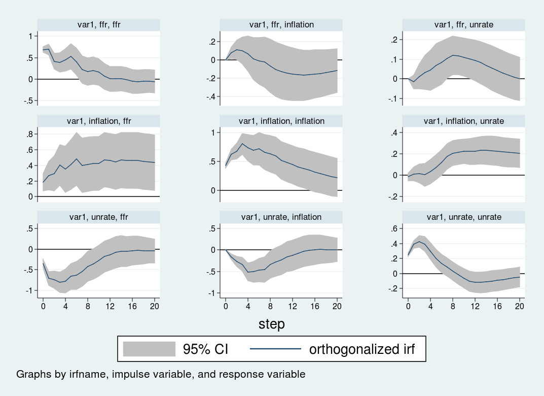
The impulse–response graph places one impulse in each row and one response variable in each column. The horizontal axis for each graph is in the units of time that your VAR is estimated in, in this case quarters; hence, the impulse–response graph shows the effect of a shock over a 20-quarter period. The vertical axis is in units of the variables in the VAR; in this case, everything is measured in percentage points, so the vertical units in all panels are percentage point changes.
The first row shows the effect of a one-standard-deviation impulse to the interest rate equation. The interest rate is persistent and remains elevated for about 12 periods (3 years) after the initial impulse. Inflation declines slightly after eight quarters, but the response is not statistically significant at any horizon. The unemployment rate rises slowly for about 12 periods, peaking at a 0.2 perentage point increase, before declining.
The second row shows the impact of a shock to the inflation equation. An unexpected increase in inflation is associated with a highly persistent increase in the unemployment rate and the interest rate. Both the interest rate and unemployment rate remain elevated even five years after the impulse to inflation.
Finally, the third row shows the impact to a shock to the unemployment equation. An impulse to the unemployment rate causes inflation to decline by about one half of one percentage point over the following year. The interest rate responds strongly to the unemployment shock, falling by nearly one percentage point over the year following the shock.
Both the VAR and the ordering used here are illustrative. All the inferences are conditional on the \(\bf{A}\) matrix, that is, the ordering of the variables in the VAR. Different orderings will produce different \(\bf{A}\) matrices, which in turn will produce different impulse responses. In addition, there are identification strategies that go beyond simply ordering the equations; I will discuss those methods in a later post.
Conclusion
In this post, I estimated a VAR model and discussed two common postestimation statistics: Granger causality tests and impulse–response functions. In my next post, I will go deeper into the impulse response function and describe alternative identification strategies for performing structural inference in a VAR.