Calculating power using Monte Carlo simulations, part 1: The basics
Power and sample-size calculations are an important part of planning a scientific study. You can use Stata’s power commands to calculate power and sample-size requirements for dozens of commonly used statistical tests. But there are no simple formulas for more complex models such as multilevel/longitudinal models and structural equation models (SEMs). Monte Carlo simulations are one way to calculate power and sample-size requirements for complex models, and Stata provides all the tools you need to do this. You can even integrate your simulations into Stata’s power commands so that you can easily create custom tables and graphs for a range of parameter values.
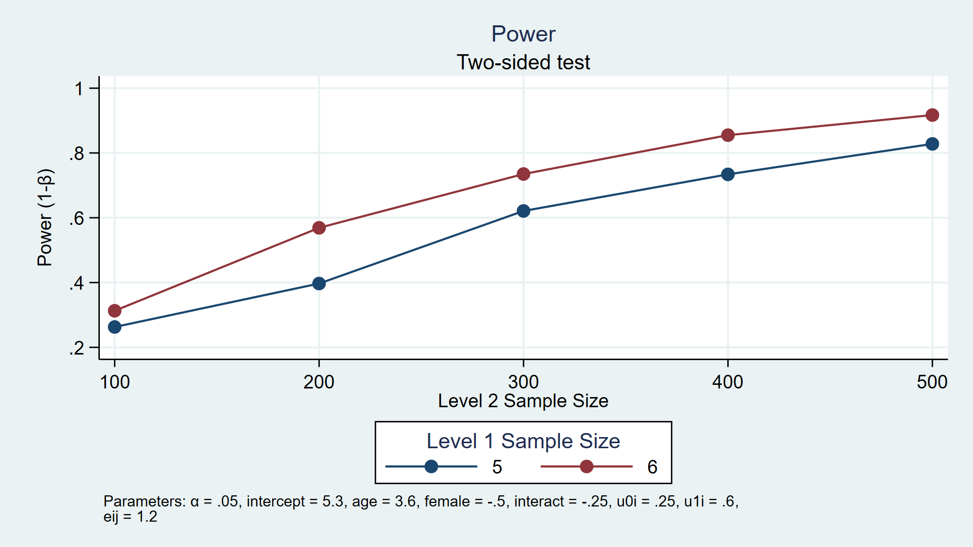
For example, the custom program power simmixed below simulates power for a longitudinal model assuming the number of participants (level 2) is 100 through 500 in increments of 100 and each participant has 5 or 6 observations (level 1). power simmixed also creates a table (not shown) and the graph below to show the results of the simulation.
power simmixed, n1(5 6) n(100(100)500) reps(1000)                           ///
      table(n1 N power)                                                     ///
      graph(ydimension(power) xdimension(N) plotdimension(n1)               ///
            xtitle(Level 2 Sample Size) legend(title(Level 1 Sample Size)))
My colleagues and I have written a series of blog posts to show you how to do this. In today’s post, I’ll introduce you to the basic tools you need to calculate power and sample-size requirements using simulations. In the second post, I’ll show you how to integrate your simulations into Stata’s power command. Then, we’ll show you specific examples for linear regression, logistic regression, multilevel/longitudinal models, and structural equation models.
The basic idea
Statistical power is the probability of rejecting the null hypothesis when the null hypothesis is false. Power is calculated based on a set of assumptions such as the sample size, the alpha level, and a specific alternative hypothesis. For example, we might wish to calculate power for a t test assuming that a sample mean is 70 for the null hypothesis, 75 for the alternative hypothesis, a sample size of 100, and an alpha level of 0.05.
The basic steps for calculating power using Monte Carlo simulations are
- to generate a dataset assuming the alternative hypothesis is true (for example, mean=75).
- to test the null hypothesis using the dataset (for example, test that the mean = 70).
- to save the results of the test (for example, “reject” or “fail to reject”).
- to repeat steps 1–3 many times (usually 1,000 or more).
The proportion of times the null hypothesis is rejected is our estimate of statistical power. In the example above, we might observe 834 “rejections” out of 1,000 iterations, which gives us an estimated power of 0.834 or 83.4%.
You will need to be familiar with some of Stata’s programming tools to perform these steps. Below is a list of topics that I will cover in this post. If you are familiar with some of these topics, you can click on the links below to skip ahead to unfamiliar topics.
List of topics
How to use program to create a simple program
How to use program to create a useful program
How to use simulate to run your program many times
Checking your results with power onemean
Scalars and local macros
Scalars and local macros are important tools for simulations because they allow you to temporarily store numbers in memory. For example, you could store the number 1 to a scalar named i by typing
. scalar i = 1
You can refer to this scalar later by typing
. display "i = " i
i = 1
Stata will become confused if you use the same name for both a scalar and a variable. You can avoid this confusion by using unique names for your scalars, or you can use the scalar() function to refer to a scalar.
. display "i = " scalar(i)
i = 1
You can also store numbers using local macros. For example, you could store the number 1 to a local macro named i by typing
. local i = 1
You can then refer to the local macro by preceding it with a left single quote (often found on the keyboard to the left of the “1” key) and following it with a right single quote (often found to the left of the Enter key).
. display "i = `i'"
i = 1
Local macros are typically used to define the input parameters of a simulation and the results of many Stata commands are stored as scalars.
Create pseudo–random datasets
You will also need to generate random numbers to conduct your simulation. Here I’ll show you a few commonly used random number functions and refer you to the Stata Functions Reference Manual for a complete list. Let’s begin by clearing Stata’s memory, setting the random number seed to 15, and using set obs to tell Stata that we would like to create a dataset with 200 observations.
. clear

. set seed 15

. set obs 200
number of observations (_N) was 0, now 200
You can use the runiform() function to generate uniformly distributed random numbers over the interval (0,1).
. generate randnum = runiform()

. list randnum in 1/5

     +----------+
     |  randnum |
     |----------|
  1. | .7827144 |
  2. | .0985331 |
  3. | .4982307 |
  4. | .7501223 |
  5. | .7992788 |
     +----------+
You can use the similar runiformint(a,b) function to generate uniformly distributed random integer variates on the interval [a,b]. For example, you could generate a random value of a person’s age on the interval [18,65] by typing the following command:
. generate age = runiformint(18,65)

. list age in 1/5

     +-----+
     | age |
     |-----|
  1. |  28 |
  2. |  61 |
  3. |  21 |
  4. |  35 |
  5. |  34 |
     +-----+
You can use the rbinomial(n,p) function to generate binomial(n,p) random variates, where n is the number of trials and p is the success probability. For example, you could generate a random indicator for female by typing the following command:
. generate female = rbinomial(1,0.5)

. list female in 1/5

     +--------+
     | female |
     |--------|
  1. |      1 |
  2. |      1 |
  3. |      0 |
  4. |      0 |
  5. |      1 |
     +--------+
You can also use the rnormal(m,s) function to generate random values from a normal density with mean equal to m and standard deviation equal to s. For example, you could generate variables for weight and height using the commands below. Here we have specified a mean of 72 kilograms and a standard deviation of 15 for weight, as well as a mean of 170 centimeters with a standard deviation of 10 for height.
. generate weight = rnormal(72,15)

. generate height = rnormal(170,10)

. list weight height in 1/5

     +---------------------+
     |   weight     height |
     |---------------------|
  1. | 66.02002   175.0715 |
  2. | 89.32963   159.6439 |
  3. | 90.97482   173.0338 |
  4. |  66.4279   185.4124 |
  5. | 74.31628   173.5268 |
     +---------------------+
In this example, we generated weight and height independently. But variables like weight and height are likely to be correlated, and you can generate correlated variables using drawnorm.
In the example below, the means are stored in the matrix m, the standard deviations in the matrix s, and the correlation between the variables in the matrix C. You can then include these matrices as arguments in the options of drawnorm to create the correlated variables height and weight.
. clear

. matrix m = (72,170)

. matrix s = (15,10)

. matrix C = (1.0, 0.5 \ 0.5, 1.0)

. drawnorm weight height, n(200) means(m) sds(s) corr(C) clear
(obs 200)

. summarize

    Variable |        Obs        Mean    Std. Dev.       Min        Max
-------------+---------------------------------------------------------
      weight |        200     71.4513     15.3586   32.01175   107.9983
      height |        200     169.728    9.642012   140.6366   193.3395
The estimates of the means and standard deviations above are similar to our input parameters, and the estimated correlation coefficient below is 0.5049, which is close to the value of 0.5 that we specified in our correlation matrix above.
. correlate
(obs=200)

             |   weight   height
-------------+------------------
      weight |   1.0000
      height |   0.5049   1.0000
Storing model output
Many Stata commands store their results as scalars, macros, and matrices. After you run a command, you can see a list of the stored results by typing return list. You can also type ereturn list after an estimation command such as regress.
In the example below, I use the ttest command to test the null hypothesis that the mean weight is equal to 70.
. ttest weight = 70

One-sample t test
------------------------------------------------------------------------------
Variable |     Obs        Mean    Std. Err.   Std. Dev.   [95% Conf. Interval]
---------+--------------------------------------------------------------------
  weight |     200     71.4513    1.086017     15.3586    69.30972    73.59288
------------------------------------------------------------------------------
    mean = mean(weight)                                           t =   1.3363
Ho: mean = 70                                    degrees of freedom =      199

    Ha: mean < 70               Ha: mean != 70                 Ha: mean > 70
 Pr(T < t) = 0.9085         Pr(|T| > |t|) = 0.1830          Pr(T > t) = 0.0915
Typing return list shows you a list of the scalars that Stata stored in memory.
. return list

scalars:
              r(level) =  95
               r(sd_1) =  15.3585990978069
                 r(se) =  1.086016957158485
                r(p_u) =  .091480506354148
                r(p_l) =  .9085194936458521
                  r(p) =  .1829610127082959
                  r(t) =  1.336349633452592
               r(df_t) =  199
               r(mu_1) =  71.45129836262204
                r(N_1) =  200
You can store any of these scalars to another scalar. For example, you could store the two-sided p-value stored in r(p) to a scalar named pvalue by typing
. scalar pvalue = r(p)

. display "The two-sided p-value is", pvalue
The two-sided p-value is .18296101
How to use program to create a simple program
You will run the commands that generate the random data and test the null hypothesis many times when you run your simulation. You will also need to define the input parameters for your simulation and return the results of your hypothesis tests. One way to do these tasks efficiently is to define your own Stata program using program. The code block below defines a program called myprogram, which accepts the input parameter n(), displays the value of n, and returns the value of n.
capture program drop myprogram
program myprogram, rclass
        version 15.1
        syntax, n(integer)
        display "n = `n'"
        return scalar N = `n'
end
Let’s consider this code block line by line.
The first line is capture program drop myprogram. Once you define a program, you must drop the program from memory using program drop before you can modify and redefine the program. Because it is likely that you will modify this program several times before you are finished, it will save time to run program drop before you redefine it. The program will not be defined the first time you run this code block, so program drop will return an error. Typing capture before program drop will capture this error and allow the code block to continue running.
The second line is program myprogram, rclass. This begins the definition of the program myprogram. After you define the program, you can type myprogram, and Stata will run all the commands between program and end. The option rclass tells Stata that we would like to return values from our program using return.
The third line, version 15.1, tells Stata that you wish to run your program using the features as written in Stata 15.1. You can learn more about version control in Stata in the Stata Programming Reference Manual.
The fourth line is syntax, n(integer). This defines the syntax of your program. The program requires the user to type a comma followed by an integer for n(). The value of n() is stored in a local macro named n, and you can refer to this local macro as `n’.
The fifth line displays the value of the local macro n.
The sixth line is return scalar N = `n’. This line instructs the program to return the value of n as a scalar named N.
The last line is end. This tells Stata that you are finished defining the program myprogram.
Let’s run myprogram and see what it does.
. myprogram, n(50)
n = 50
I entered a value of 50 for n(), and Stata displayed the result n = 50.
I can type return list and see that myprogram returns the value of n as the scalar r(N).
. return list

scalars:
                  r(N) =  50
It works!
How to use program to create a useful program
Let’s define a program called simttest that generates a random dataset based on input parameters, tests the null hypothesis, and returns the results of our hypothesis test. The code block below defines the program using only comments.
program simttest, rclass
    version 15.1
    // DEFINE THE INPUT PARAMETERS AND THEIR DEFAULT VALUES

    // GENERATE THE RANDOM DATA AND TEST THE NULL HYPOTHESIS

    // RETURN RESULTS
end
Now, let’s fill in the details in the code block below.
capture program drop simttest
program simttest, rclass
    version 15.1

    // DEFINE THE INPUT PARAMETERS AND THEIR DEFAULT VALUES
    syntax, n(integer)          ///  Sample size
          [ alpha(real 0.05)    ///  Alpha level
            m0(real 0)          ///  Mean under the null
            ma(real 1)          ///  Mean under the alternative
            sd(real 1) ]        //   Standard deviation

    // GENERATE THE RANDOM DATA AND TEST THE NULL HYPOTHESIS
    drawnorm y, n(`n') means(`ma') sds(`sd') clear
    ttest y = `m0'

    // RETURN RESULTS
    return scalar reject = (r(p)<`alpha')
end
The definition of syntax includes one required parameter, n(), and four optional parameters, alpha(), m0(), ma(), and sd(). The optional parameters are enclosed in square brackets. All the input parameters include a restriction on the input values. For example, n() must be an integer, and the optional parameters must be real numbers. The optional parameters also include a default value that is used if users do not specify the input parameter when they type the program name. For example, m0 will be assigned a value of 0 unless users specify a different value.
Note that in this example n() is the sample size, alpha() is the alpha level, m0() is the mean assuming the null hypothesis, ma() is the mean assuming the alternative hypothesis, and sd() is the standard deviation.
The input parameters are then used by drawnorm to generate a sample with `n’ observations from a normal distribution with a mean of `ma’ and a standard deviation of `sd’. Next, ttest tests the null hypothesis that the sample mean equals `m0′.
You can return the results of the hypothesis test by typing return scalar reject = (r(p)<`alpha'). Recall that ttest stores the two-sided p-value in the scalar r(p). Our program returns a value of 1 using the scalar reject when r(p) is less than the alpha level specified by `alpha’ and 0 otherwise.
Now, you can type simttest along with the input parameters to run the simulation.
. simttest, n(100) m0(70) ma(75) sd(15) alpha(0.05)
(obs 100)

One-sample t test
------------------------------------------------------------------------------
Variable |     Obs        Mean    Std. Err.   Std. Dev.   [95% Conf. Interval]
---------+--------------------------------------------------------------------
       y |     100    77.22324    1.597794    15.97794    74.05287    80.39361
------------------------------------------------------------------------------
    mean = mean(y)                                                t =   4.5208
Ho: mean = 70                                    degrees of freedom =       99

    Ha: mean < 70               Ha: mean != 70                 Ha: mean > 70
 Pr(T < t) = 1.0000         Pr(|T| > |t|) = 0.0000          Pr(T > t) = 0.0000
You can see the results of the simulation by typing return list.
. return list

scalars:
             r(reject) =  1
How to use simulate to run your program many times
The program simttest will do everything you need for one iteration of your simulation. Next, you will need a way to run simttest many times and collect the results. The code block below shows how to use simulate to accomplish both of these tasks.
simulate reject=r(reject), reps(100) seed(12345):              ///
         simttest, n(100) m0(70) ma(75) sd(15) alpha(0.05)
The argument reject=r(reject) tells simulate to save the results returned in r(reject) to a variable named reject. The option reps(100) instructs simulate to run your program 100 times. The option seed(12345) sets the random number seed so that our results will be reproducible.
The colon is followed by simttest along with the input parameters for our simulation. Some simulations take a long time to run, and simulate displays a dot in the results window so that you know it is still running. The output below shows the results of our simulation.
. simulate reject=r(reject), reps(100) seed(12345):       ///
>         simttest, n(100) m0(70) ma(75) sd(15) alpha(0.05)

      command:  simttest, n(100) m0(70) ma(75) sd(15) alpha(0.05)
       reject:  r(reject)

Simulations (100)
----+--- 1 ---+--- 2 ---+--- 3 ---+--- 4 ---+--- 5
..................................................    50
..................................................   100
simulate saved the results to the variable reject, which contains a 1 if the test of the null hypothesis was rejected and 0 otherwise.
. list in 1/5

     +--------+
     | reject |
     |--------|
  1. |      1 |
  2. |      1 |
  3. |      1 |
  4. |      0 |
  5. |      1 |
     +--------+
You can use summarize to calculate the mean of reject, which equals the proportion of times out of 100 iterations that the null hypothesis was rejected. That proportion is your estimate of statistical power given the input parameters!
. summarize reject

    Variable |        Obs        Mean    Std. Dev.       Min        Max
-------------+---------------------------------------------------------
      reject |        100         .91    .2876235          0          1
In this example, the proportion equals 0.91, which means that you can expect 91% power when testing the alternative hypothesis that the sample mean equals 75 against the null hypothesis that the sample mean equals 70 given a standard deviation of 15 and a sample size of 100. In practice, you would want to increase the number of repetitions to 1,000 or even 10,000. You could also vary the sample size and other input parameters to explore their effects on power.
Checking your results with power onemean
We can check the results of our Monte Carlo simulation using power onemean. The example below includes the same input parameters as our simulation.
. power onemean 70 75, n(100) sd(15)

Estimated power for a one-sample mean test
t test
Ho: m = m0  versus  Ha: m != m0

Study parameters:

        alpha =    0.0500
            N =       100
        delta =    0.3333
           m0 =   70.0000
           ma =   75.0000
           sd =   15.0000

Estimated power:

        power =    0.9100
The power calculated by power onemean equals 0.9100, which is the same as the power estimated by our simulation. The results won’t always argee perfectly because simulations are random. Changing the random number seed or the number of iterations may change the estimated power slightly. But the results should be close.
Summary
In this post, I introduced the tools you will need to calculate statistical power and sample-size requirements using Monte Carlo simulations. Next time, I will show you how to use Stata’s power command to run your simulations so that you can easily create tables and graphs for a range of input parameters.