Prediction intervals with gradient boosting machine
Introduction
Machine learning methods, such as ensemble decision trees, are widely used to predict outcomes based on data. However, these methods often focus on providing point predictions, which limits their ability to quantify prediction uncertainty. In many applications, such as healthcare and finance, the goal is not only to predict accurately but also to assess the reliability of those predictions. Prediction intervals, which provide lower and upper bounds such that the true response lies within them with high probability, are a reliable tool for quantifying prediction accuracy. An ideal prediction interval should meet several criteria: it should offer valid coverage (defined below) without relying on strong distributional assumptions, be informative by being as narrow as possible for each observation, and be adaptive—provide wider intervals for observations that are “difficult” to predict and narrower intervals for “easy” ones.
You may wonder whether it’s possible to construct a statistically valid prediction interval using any machine learning method, without any distributional assumption such as Gaussianity, while the above criteria are satisfied. Wait and see.
In this post, I demonstrate how to use Stata’s h2oml suite of commands to construct predictive intervals by using the conformalized quantile regression (CQR) approach, introduced in Romano, Patterson, and Candes (2019). The structure of the post is as follows: First, I provide a brief introduction to conformal prediction, with a focus on CQR, and then I show how to construct predictive intervals in Stata by using gradient boosting regressions.
Conformal prediction
Conformal prediction (Papadopoulos et al. 2002; Vovk, Gammerman, and Shafer 2005; Lei et al. 2018; Angelopoulos and Bates 2023), also known as conformal inference, is a general methodology designed to complement any machine learning prediction by providing prediction intervals with guaranteed distribution-free statistical coverage. At a conceptual level, conformal prediction starts with a pretrained machine learning model (for example, a gradient boosting machine) trained on exchangeable or independent and identically distributed data. It then uses held-out validation data from the same data-generating distribution, referred to as calibration data, to define a score function \(S(\hat y, y)\). This function assigns larger scores when the discrepancy between the predicted value \(\hat y\) and the true response \(y\) is greater. These scores are subsequently used to construct prediction intervals for new, unseen observations \({\bf X}_{\text{new}}\), where \({\bf X}_{\text{new}}\) is a random vector of predictors.
It can be shown that conformal prediction \(\mathcal{C}({\bf X}_{\text{new}})\) provides valid prediction interval coverage (Lei et al. 2018; Angelopoulos and Bates 2023) in the sense that
\[
P\{Y_{\text{new}} \in \mathcal{C}({\bf X}_{\text{new}})\} \geq 1 – \alpha \tag{1}\label{eq1}
\]
where \(\alpha \in (0,1)\) is a user-defined miscoverage or error rate. This property is called marginal coverage, because the probability is averaged over the randomness of calibration and unseen or testing data.
Although the conformal prediction approach guarantees valid coverage \eqref{eq1} with minimal distributional assumptions and for any machine learning method, our focus here is on CQR (Romano, Patterson, and Candes 2019). It is one of the most widely used and recommended approaches to construct prediction intervals (Romano, Patterson, and Candes 2019; Angelopoulos and Bates 2023).
CQR
The exposure in this section closely follows Romano, Patterson, and Candes (2019) and Angelopoulos and Bates (2023). Consider a quantile regression that estimates a conditional quantile function \(q_{\alpha}(\cdot)\) of \(Y_{\text{new}}\) given \({\bf X}_{\text{new}} = {\bf x}\) for each possible realization of \({\bf x}\). We can use any quantile regression estimation method, such as gradient boosting machine with quantile or “pinball” loss to obtain \(\widehat q_{\alpha}(\cdot)\). By definition, \(Y_{\text{new}}|{\bf X}_{\text{new}} = {\bf x}\) is below \(q_{\alpha/2}({\bf x})\) with probability \(\alpha/2\) and above \(q_{1 – \alpha/2}({\bf x})\) with probability \(\alpha/2\), so the estimated prediction interval \([\widehat q_{\alpha/2}(\cdot), \widehat q_{1 – \alpha/2}(\cdot)]\) should have approximately \(1-\alpha\)% coverage. Unfortunately, because the estimated quantiles can be inaccurate, such coverage is not guaranteed. Thus, we need to conformalize them to have a valid coverage \eqref{eq1}. CQR steps can be summarized as follows:
- Step 1. Split data \(\mathcal{D}\) into a training \(\mathcal{D}_1\) and calibration \(\mathcal{D}_2\), and let \(\mathcal{D}_3\) be the new, unseen testing data.
- Step 2. Use \(\mathcal{D}_1\) to train any quantile regression estimation method \(f\) to estimate two conditional quantile functions \(\hat q_{\alpha_1}(\cdot)\) and \(\hat q_{\alpha_2}(\cdot)\), for \(\alpha_1 = \alpha/2\) and \(\alpha_2 = 1 – \alpha/2\), respectively. For example, when the miscoverage rate \(\alpha = 0.1\), we obtain \(\hat q_{0.05}(\cdot)\) and \(\hat q_{0.95}(\cdot)\).
- Step 3. Use calibration data \(\mathcal{D}_2\) to compute conformity scores \(S_i\), for each \(i \in \mathcal{D}_2\), that quantify the error made by the interval \([\hat q_{\alpha_1}({\bf x}), \hat q_{\alpha_2}({\bf x})]\).
\[
S_i = \max \{\hat q_{\alpha_1}({\bf x}_i) – Y_i, Y_i – \hat q_{\alpha_2}({\bf x}_i)\}
\] - Step 4. Given new unseen data \({\bf X}_{\text{new}} \subset \mathcal{D}_3\), construct the prediction interval for \(Y_{\text{new}}\),
\[
\mathcal{C}({\bf X}_{\text{new}}) = \Big[\hat q_{\alpha_1}({\bf X}_{\text{new}}) – q_{1 – \alpha}(S_i, \mathcal{D}_2), \hat q_{\alpha_2}({\bf X}_{\text{new}}) + q_{1 – \alpha}(S_i, \mathcal{D}_2)\Big]
\]
where the empirical quantile of conformity scores
\[ \label{eq:empquantile}
q_{1 – \alpha}(S_i, \mathcal{D}_2) = \frac{\lceil (|\mathcal{D}_2|+1)(1 – \alpha) \rceil}{|\mathcal{D}_2|} \tag{2}
\]
and \(|\mathcal{D}_2|\) is the number of observations of the calibration data and \(\lceil \cdot \rceil\) is the ceiling function.
The intuition behind the conformity score, computed in step 3, is the following:
- If \(Y_{\text{new}} < q_{\alpha_1}({\bf X}_{\text{new}})\) or \(Y_{\text{new}} > q_{\alpha_2}({\bf X}_{\text{new}})\), the scores given by \(S_i = |Y_{\text{new}} – q_{\alpha_1}({\bf X}_{\text{new}})|\) or \(S_i = |Y_{\text{new}} – q_{\alpha_2}({\bf X}_{\text{new}})|\) represent the magnitude of the error incurred by this mistake.
- On the other hand, if \(q_{\alpha_1}({\bf X}_{\text{new}}) \leq Y_{\text{new}} \leq q_{\alpha_2}({\bf X}_{\text{new}})\), the computed score is always nonpositive.
This way, the conformity score accounts for both undercoverage and overcoverage.
Romano, Patterson, and Candes (2019) showed that under the exchangeability assumption, steps 1–4 guarantee the valid marginal coverage \eqref{eq1}.
Implementation in Stata
In this section, we use the h2oml suite of commands in Stata to construct predictive intervals using conformalized gradient boosting quantile regression. H2O is a scalable and distributed machine learning and predictive analytics platform that allows us to perform data analysis and machine learning. For details, see the Stata 19 Machine Learning in Stata Using H2O: Ensemble Decision Trees Reference Manual.
We consider the Ames housing dataset (De Cock 2011), ameshouses.dta, also used in a Kaggle competition, which describes residential houses sold in Ames, Iowa, between 2006 and 2010. It contains about 80 housing (and related) characteristics, such as home size, amenities, and location. This dataset is often used for building predictive models for home sale price, saleprice. Before putting the dataset into an H2O frame, we perform some data manipulation in Stata. Because saleprice is right-skewed (for example, type histogram saleprice), we use its log. We also generate a variable, houseage, that calculates the age of the house at the time of a sales transaction.
. webuse ameshouses

. generate logsaleprice = log(saleprice)

. generate houseage = yrsold - yearbuilt

. drop saleprice yrsold yearbuilt
Next, we initialize a cluster and put the data into an H2O frame. Then, to perform step 1, let’s split the data into training (50%), calibration (40%), and testing (10%) frames, where the testing frame serves as a proxy for new, unseen data.
. h2o init
(output omitted)

. _h2oframe put, into(house)

Progress (%): 0 100

. _h2oframe split house, into(train calib test) split(0.5 0.4 0.1)
> rseed(1)

. _h2oframe change train
Our goal is to construct a predictive interval with 90% coverage. We define three local macros in Stata to store the miscoverage rate \(\alpha = 1- 0.9 = 0.1\) and lower and upper bounds, \(0.05\) and \(0.95\), respectively. Let’s also create a global macro, predictors, that contains the names of our predictors.
. local alpha = 0.1

. local lower = 0.05

. local upper = 0.95

. global predictors overallqual grlivarea exterqual houseage garagecars
> totalbsmtsf stflrsf garagearea kitchenqual bsmtqual
We perform step 2 by pretraining gradient boosting quantile regression by using the h2oml gbregress command with the loss(quantile) option. For illustration, I tune only the number of trees (ntrees()) and maximum-depth (maxdepth()) hyperparameters, and store the estimation results by using the h2omlest store command.
. h2oml gbregress logsaleprice $predictors, h2orseed(19) cv(3, modulo)
> loss(quantile, alpha(`lower')) ntrees(20(20)80) maxdepth(6(2)12)
> tune(grid(cartesian))

Progress (%): 0 100

Gradient boosting regression using H2O

Response: logsaleprice
Loss:     Quantile .05
Frame:                                 Number of observations:
  Training: train                                 Training =    737
                                          Cross-validation =    737
Cross-validation: Modulo               Number of folds     =      3

Tuning information for hyperparameters

Method: Cartesian
Metric: Deviance

-------------------------------------------------------------------
                 |                      Grid values
 Hyperparameters |         Minimum          Maximum        Selected
-----------------+-------------------------------------------------
 Number of trees |              20               80              40
 Max. tree depth |               6               12               8
-------------------------------------------------------------------

Model parameters

Number of trees      =  40             Learning rate       =     .1
              actual =  40             Learning rate decay =      1
Tree depth:                            Pred. sampling rate =      1
           Input max =   8             Sampling rate       =      1
                 min =   6             No. of bins cat.    =  1,024
                 avg = 7.5             No. of bins root    =  1,024
                 max =   8             No. of bins cont.   =     20
Min. obs. leaf split =  10             Min. split thresh.  = .00001
Metric summary
-----------------------------------
           |                 Cross-
    Metric |   Training  validation
-----------+-----------------------
  Deviance |   .0138451    .0259728
       MSE |   .1168036    .1325075
      RMSE |   .3417654    .3640158
     RMSLE |   .0259833    .0278047
       MAE |   .2636412    .2926809
 R-squared |   .3117896    .2192615
-----------------------------------

. h2omlest store q_lower
The best-selected model has 40 trees and a maximum tree depth of 8. I use this model to obtain predicted lower quantiles on the calibration dataset by using the h2omlpredict command with the frame() option. We will use those predicted values to compute conformity scores in step 3.
. h2omlpredict q_lower, frame(calib)

Progress (%): 0 100
For simplicity, I use the above hyperparameters to run gradient boosting quantile regression for the upper quantile. In practice, we need to tune hyperparameters for this model as well. As before, I predict the upper quantiles on the calibration dataset and store the model.
. h2oml gbregress logsaleprice $predictors, h2orseed(19) cv(3, modulo)
> loss(quantile, alpha(`upper')) ntrees(40) maxdepth(8)

Progress (%): 0 1.2 100

Gradient boosting regression using H2O

Response: logsaleprice
Loss:     Quantile .95
Frame:                                 Number of observations:
  Training: train                                 Training =    737
                                          Cross-validation =    737
Cross-validation: Modulo               Number of folds     =      3

Model parameters

Number of trees      =  40             Learning rate       =     .1
              actual =  40             Learning rate decay =      1
Tree depth:                            Pred. sampling rate =      1
           Input max =   8             Sampling rate       =      1
                 min =   5             No. of bins cat.    =  1,024
                 avg = 7.2             No. of bins root    =  1,024
                 max =   8             No. of bins cont.   =     20
Min. obs. leaf split =  10             Min. split thresh.  = .00001

Metric summary
-----------------------------------
           |                 Cross-
    Metric |   Training  validation
-----------+-----------------------
  Deviance |   .0132103    .0218716
       MSE |   .1190689    .1365112
      RMSE |   .3450637    .3694742
     RMSLE |   .0268811    .0287084
       MAE |   .2567844    .2841911
 R-squared |   .2984421    .1956718
-----------------------------------

. h2omlest store q_upper

. h2omlpredict q_upper, frame(calib)

Progress (%): 0 100
To compute conformity scores as in step 3, let’s use the _h2oframe get command to load the estimated quantiles and the logarithm of the sales price from the calibration frame calib into Stata. Because the data in Stata’s memory have been modified, I also use the clear option.
. _h2oframe get logsaleprice q_lower q_upper using calib, clear
Then, we use those variables to generate a new variable, conf_scores, that contains the computed conformity scores.
. generate double conf_scores =
> max(q_lower - logsaleprice, logsaleprice - q_upper)
To construct conformalized prediction intervals from step 4, we need to compute empirical quantiles \eqref{eq:empquantile}, which can be done in Stata by using the _pctile command. Figure 1a shows the distribution of conformity scores, and the red vertical line indicates the empirical quantile \eqref{eq:empquantile}, which is equal to 0.031.
. local emp_quantile = ceil((1 - 0.1) * (_N + 1))/ _N * 100

. _pctile conf_score, percentiles(`emp_quantile')

. local q = r(r1)

. di `q'
.03104496
Next, I restore both models that estimated lower and upper quantiles and obtain their predictions on the testing frame test.
. h2omlest restore q_lower
(results q_lower are active now)

. h2omlpredict q_lower, frame(test)

Progress (%): 0 100

. h2omlest restore q_upper
(results q_upper are active now)

. h2omlpredict q_upper, frame(test)

Progress (%): 0 100
I then load those predictions from the testing frame into Stata and generate lower and upper bounds for prediction intervals. In addition, I also load the logsaleprice and houseage variables. We will use those variables for illustration purposes.
. _h2oframe get logsaleprice houseage q_lower q_upper using test, clear

. generate double conf_lower = q_lower - `q'

. generate double conf_upper = q_upper + `q'
Figure 1b displays the prediction intervals for each observation in the testing frame. We can see that the computed interval is adaptive, meaning for “difficult” observations, for example, outliers, the interval is wide and vice versa.
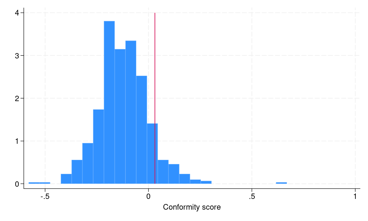 (a) Histogram of conformity scores |
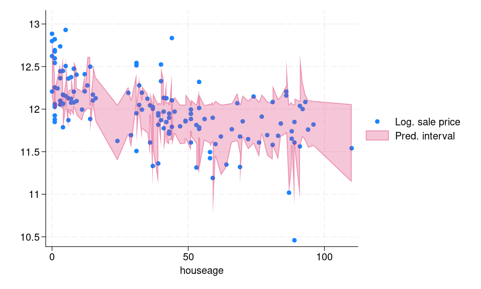 (b) Prediction intervals for the testing dataset |
|
Figure 1: (a) Histogram of conformity scores (b) CQR-based prediction intervals for the testing dataset |
|
Below, I list a small sample of the prediction intervals and the true log of sale price response.
. list logsaleprice conf_lower conf_upper in 1/10

     +----------------------------------+
     | logsal~e   conf_lo~r   conf_up~r |
     |----------------------------------|
  1. | 11.67844   11.470275   12.052485 |
  2. |  12.6925   12.002838   12.773621 |
  3. | 11.31447   11.332932   12.058372 |
  4. | 11.64833   11.527202   12.099679 |
  5. | 12.10349   11.640463   12.401743 |
     |----------------------------------|
  6. |  11.8494   11.621721   12.231588 |
  7. |  11.8838   11.631179   12.045645 |
  8. | 12.06681   11.931026   12.204194 |
  9. | 12.12811   11.852887   12.375453 |
 10. | 11.65269   11.569664   12.066292 |
     +----------------------------------+
For 9 out of 10 observations, the responses belong to the respective predictive intervals. We can compute the actual average coverage of the interval in the testing frame, which I do next by generating a new variable, in_interval, that indicates whether the response logsaleprice is in the prediction interval.
. generate byte in_interval = 0

. replace in_interval = 1 if inrange(logsaleprice, conf_lower, conf_upper)
(124 real changes made)

. summarize in_interval, meanonly

. local avg_coverage = r(mean)

. di `avg_coverage' * 100
90.510949
We can see that the actual average coverage is 90.5%.
References
Angelopoulos, A. N., and S. Bates. 2023. Conformal prediction: A gentle introduction. Foundations and Trends in Machine Learning 16: 494–591. https://doi.org/10.1561/2200000101.
De Cock, D. 2011. Ames, Iowa: Alternative to the Boston housing data as an end of semester regression project. Journal of Statistics Education 19: 3. https://doi.org/10.1080/10691898.2011.11889627.
Lei, J., M. G’Sell, A. Rinaldo, R. J. Tibshirani, and L. Wasserman. 2018. Distribution-free predictive inference for regression. Journal of the American Statistical Association 113: 1094–1111. https://doi.org/10.1080/01621459.2017.1307116.
Papadopoulos, H., K. Proedrou, V. Vovk, and A. Gammerman. 2002. “Inductive confidence machines for regression”. In Machine Learning: ECML 2002. Lecture Notes in Computer Science, edited by T. Elomaa, H. Mannila, H. Toivonen, vol. 2430: 345–356. Berlin: Springer. https://doi.org/10.1007/3-540-36755-1_29.
Romano, Y., E. Patterson, and E. Candes. 2019. “Conformalized quantile regression”. In Advances in Neural Information Processing Systems, edited by H. Wallach, H. Larochelle, A. Beygelzimer, F. d’Alché-Buc, E. Fox, and R. Garnett, vol. 32. Red Hook, NY: Curran Associates, Inc. https://proceedings.neurips.cc/paper_files/paper/2019/file/5103c3584b063c431bd1268e9b5e76fb-Paper.pdf.
Vovk, V., A. Gammerman, and G. Shafer. 2005. Algorithmic Learning in a Random World. New York: Springer. https://doi.org/10.1007/b106715.