Training or testing? Which dataset should you use to explain your model?
The h2oml suite of commands in Stata provides several postestimation commands for explaining machine learning models. You often have a choice of which dataset to use for the explanation, and that choice can affect your results. In this post, we use a simulated example to examine that choice and provide recommendations for practitioners.
Motivation
Suppose you have fit a gradient boosting model with h2oml gbregress, and you now want to know which predictors are important. You type
. h2omlgraph permimp
and you get a ranking of your predictors. One of them, a predictor you included only because it happened to be in the dataset, received a clearly nonzero importance. Perhaps it matters more than you thought.
Now you type almost the same thing but on the testing dataset,
. h2omlgraph permimp, test
and that same predictor’s importance drops to a fraction of what it was. Note that nothing about the model changed between those two commands. The only difference is the dataset that the importance was computed on.
So which number should you report? The answer turns out to be different for different explainability commands, and that is what this post is about. We summarize our suggestions in table 6 at the end.
The question of which dataset to use is not new. It is asked and partly answered in the interpretable machine learning literature, most recently by Heiß et al. (2026), who derive a mean squared error decomposition for predictor effect estimates and study which dataset should be used to compute them. Molnar (2025) examined the same question for permutation importance. In this post, we set up a small simulated example in Stata where the correct answer is known exactly and then use the h2oml suite of commands to explore those claims.
What the explainability commands actually tell you
Before you choose a dataset, it helps to be clear about what each command is computing, because the command’s answer is designed to answer different questions. If you are already familiar with these commands, you can skip ahead to the next section.
Partial dependence and individual conditional expectation
h2omlgraph pdp, documented in [H2OML] h2omlgraph pdp, draws the average relationship between predictors and the prediction (Friedman 2001). It works by taking each observation in the frame, replacing the predictors of interest with a grid value, keeping everything else about that observation fixed, and asking the model for a prediction. Averaging those predictions over all observations gives one point on the curve. Repeating over a grid provides the curve.
h2omlgraph ice, documented in [H2OML] h2omlgraph ice, does the same thing without the averaging, drawing one curve per observation (Goldstein et al. 2015). As we will see, averaging, compared with individual curves, can hide heterogeneity in the dataset.
Variable importance
h2omlgraph varimp, documented in [H2OML] h2omlgraph varimp, reports how much each predictor contributed to the tree-building process. Every time a tree splits on a predictor, the split reduces the prediction error by some amount, and those reductions are added up over all trees (Breiman 2001; Friedman 2001). A predictor that the trees split on often gets a high score.
This is sometimes called split-based or impurity-based importance and is computed while the trees are being grown. It is also known to favor predictors that contain many possible split points, such as continuous predictors and categorical predictors with many levels, even when those predictors are not important (Strobl et al. 2007).
Permutation importance
h2omlgraph permimp, documented in [H2OML] h2omlgraph permimp, takes a different approach and was originally introduced by Breiman (2001). It takes a fitted model, shuffles the values of one predictor so that any relationship with the response is destroyed, and measures how much worse the predictions get. A predictor whose shuffling significantly reduces the prediction performance is important and is unimportant otherwise. Note that this requires computing a performance metric, which requires data with known responses.
SHAP values
h2omlgraph shapvalues, documented in [H2OML] h2omlgraph shapvalues, is designed to answer a question about one specific observation. Given this customer, this patient, or this loan application, how did each predictor push the prediction up or down relative to the average prediction? The values are computed using a method from cooperative game theory (Lundberg and Lee 2017), with an efficient implementation for tree ensembles (Lundberg et al. 2020). h2omlgraph shapsummary draws the same quantity for many observations at once, which gives a picture of what the model is doing overall.
Why the choice of dataset matters
Before we proceed, let us look at how the commands work with different datasets, shown in table 1. Several of the h2oml postestimation commands accept the train, valid, test, and frame() options to specify the dataset, and there is a convenience command, h2omlpostestframe, for setting a default dataset. The h2oml commands work with data stored in the H2O cluster as H2O frames, so the training, validation, and testing datasets are each an H2O frame. To be consistent with this terminology, from here on we use the word “frame” to refer to a dataset.
Table 1: Frame support across the h2oml explainability commands, as documented in [H2OML] h2oml postestimation.
| Command | train/valid/test/frame() | Honors h2omlpostestframe |
|---|---|---|
| h2omlgraph varimp | no | no |
| h2omlgraph permimp | yes | yes |
| h2omlgraph pdp | yes | yes |
| h2omlgraph ice | yes | yes |
| h2omlgraph shapvalues | yes | yes |
| h2omlgraph shapsummary | yes | yes |
We see that h2omlgraph varimp has no frame option at all. That is not an oversight. Impurity-based importance is accumulated while the trees are grown, so it can only ever describe what happened during training. Every other postestimation command in the table computes results after the model is fit.
A simulated example
To be able to examine which frame gives a better answer, we need to know what the right answer is. Real data will not tell us. Thus, we rely on simulation.
Our data are generated by
\begin{equation}
y = 4\sin(1.5 x_1) + 2 x_2 + 3 x_4 (2g-1) + \varepsilon,
\qquad \varepsilon \sim N(0, 1.5^2)
\tag{1}
\end{equation}
where \(x_1 \sim U(-3,3)\), \(x_2 \sim N(0,1)\), \(x_4 \sim U(-2,2)\), and \(g\) is a coin flip taking values 0 and 1. We include three more predictors that do not appear in (1) at all.
- \(x_3\) is correlated with \(x_2\) at 0.9 but has no effect of its own. Such variables are common in practice, and they are a standard difficulty for explainability methods (Hooker et al. 2021; Apley and Zhu 2020).
- \(x_5\) is drawn from \(U(0,1)\) and is pure noise. Being continuous, it offers the trees many possible split points.
- \(x_6\) is a coin flip and is also pure noise. It offers the trees only one split point, which makes it a useful control for \(x_5\).
To generate data, we type in Stata
. clear
. set seed 20260729
. set obs 4000
. generate double x1 = runiform(-3, 3)
. generate double x2 = rnormal()
. generate double x3 = 0.9*x2 + sqrt(1 - 0.9^2)*rnormal()
. generate double x4 = runiform(-2, 2)
. generate byte   g  = runiform() < 0.5
. generate double x5 = runiform()
. generate byte   x6 = runiform() < 0.5
. generate double y  = 4*sin(1.5*x1) + 2*x2 + 3*x4*(2*g - 1) + rnormal(0, 1.5)
In this post, every result we provide is complemented with the do-file that produced it, and the file name appears in the caption of each table and figure. Each file is self-contained, so it starts the H2O cluster, simulates its own data, and reproduces that one result from beginning to end.
In the data-generation process, \(x_1\) enters on its own, while \(x_4\) is an interaction term that enters only in combination with \(g\). When \(g = 1\), the effect of \(x_4\) is \(+3\) per unit, and \(-3\) when \(g = 0\). Heiß et al. (2026) show that the estimation variance of a partial dependence estimate is driven by the variability of the individual curves that get averaged, which in turn depends on whether the predictor interacts with other predictors. Therefore, their theory predicts that the frame should matter for \(x_4\) and much less for \(x_1\). Having both in the same simulation lets us check that claim.
The design also gives us the true partial dependence curves exactly, which is what lets us measure the error of an estimate. Because \(x_2\), \(x_4\), and \(2g-1\) all have mean zero, averaging (1) over all predictors except the predictor of interest gives
\begin{equation}
\mathrm{PD}(x_1) = 4\sin(1.5x_1), \qquad
\mathrm{PD}(x_2) = 2x_2, \qquad
\mathrm{PD}(x_4) = 0 \tag{2}
\end{equation}
exactly. Note that the true partial dependence of \(x_4\) is a flat line at zero, even though \(x_4\) has one of the largest effects in the model. The two subgroups defined by \(g\) have effects of equal size and opposite sign, so they cancel in the average. Thus, any departure from 0 in an estimated \(\mathrm{PD}(x_4)\) curve is pure error, and we can measure it.
Setting up the H2O frames
We start the H2O cluster, put the simulated data into an H2O frame, and split it into training, validation, and test frames.
. h2o init
. _h2oframe put, into(all)
. _h2oframe split all, into(train valid test) split(0.6 0.2 0.2) rseed(19)
. _h2oframe change train
That leaves about 2,400 observations in train and about 800 in each of valid and test. The proportions are applied at random rather than exactly, meaning that the realized sizes depend on rseed(). For details, see _h2oframe split.
In practice, the model is fit on train. The validation frame valid is used while the model is still being developed, for comparing candidate specifications of hyperparameters or for stopping the estimation early. The test frame is held back and looked at once, after the model is settled, so that it measures performance on data that have not been used in any choice you made during model development. See the three-way holdout method in [H2OML] Intro.
We will also use the training and validation observations together in a single frame to test one of the recommendations in Heiß et al. (2026). To append those frames rowwise, we use the _h2oframe rbind command.
. _h2oframe rbind train valid, into(trainvalid)
The into() option sends the result to a new frame named trainvalid. For details, see _h2oframe rbind. We now have 4 frames to work with, train, valid, test, and trainvalid, the last holding about 3,200 observations.
Next we fit a model. The code for this section is in setup_metrics.do.
. h2oml gbregress y x1 x2 x3 x4 g x5 x6, validframe(valid)
> ntrees(500) maxdepth(12) minobsleaf(1) lrate(0.1) h2orseed(19)
(output omitted)
Specifying 500 deep trees with as few as 1 observation per leaf lets the model memorize the training data. We can see that the training mean squared error is \(2.5\times 10^{-11}\) with an \(R^2\) of 1.000, against a validation mean squared error of 8.37 and an \(R^2\) of 0.676. Because the noise in (1) has variance \(1.5^2 = 2.25\), even a perfect model could not get the validation error below about 2.25, so 8.37 is 3.7 times that.
We overfit the above model on purpose, because it is the hardest case for the claim that training frame explanations are trustworthy. Later, we ask what changes when the model is tuned properly.
Partial dependence and the choice of frame
Heiß et al. (2026) show that although test data are theoretically the cleaner choice for estimating predictor effects, the bias from using training data is empirically negligible and is outweighed by the larger sample size that training data usually offers. Because from (2) we know the true partial dependence curves, we can examine this claim.
We hold the fitted model fixed and vary only the frame that the partial dependence is averaged over. Any difference in accuracy is then attributable to the frame and not to the model.
Note that comparing the training frame against the testing frame would not answer the question on its own, because those two frames differ in two ways simultaneously. First, they contain different observations, training dataset in one case and unseen test dataset in the other, and, second, they contain different numbers of observations, 2,400 against 800. If the training frame produced the better curve, we could not say whether that happened because the observations were training or simply because there were three times as many of them. Because the claim in Heiß et al. (2026) is precisely that the first effect exists but is outweighed by the second, a comparison that cannot tell them apart is biased.
To overcome this, we vary one of the two at a time. We start by varying the sample size while holding the type of data fixed, by dividing the testing data into subsets of increasing size. The same two commands from above do the work, splitting the testing frame into quarters and then rebuilding the larger subsets from them.
. _h2oframe split test, into(q1 q2 q3 q4) split(0.25 0.25 0.25 0.25) rseed(19)
. _h2oframe rbind q1 q2, into(h400)
This gives us three frames of increasing size, namely, q1 with about 200 observations, h400 with about 400, and test itself with about 800. Because the quarters are assigned at random, those sizes are approximate. The three are nested by construction, because q1 is part of h400, which is part of test. This is important because it means moving along the series adds observations without exchanging any, so a change in accuracy reflects the extra observations and not the luck of a different draw. The model never saw any of them, so the type of data stays the same throughout, and only the size varies.
Therefore, comparing accuracy across these three frames shows what extra observations alone are contributing, and that determines the expectation for the training frame, which holds about 2,400 observations. If reusing training data for explanation carries a significant penalty, the training frame will be less accurate than that expectation, and the improvement seen across the three holdout frames will stall or reverse. If the penalty is negligible, the training frame will be more accurate than the largest holdout, and the improvement will continue as we add more observations. Thus, we are not looking for a particular number but rather the direction of the change as we increase the sample size in the testing frame.
We repeat the above steps 15 times, generating fresh data in each replication. Each cell of table 2 is the root mean squared difference between the estimated partial dependence curve and the true curve in (2), taken over 20 points of a common grid and averaged over the replications. Both curves are centered first, and a value of zero means the estimate recovers the curve exactly. We also report the realized size of each frame, because the split does not divide the data exactly. For the code, see pd_frames.do.
Table 2: RMSE of the centered partial dependence against the truth in (2), averaged over 15 replications. The model is refit in each replication but is the same across frames within a replication. All frames are scored on one common grid, \(x_1 \in [-2.8, 2.8]\) and \(x_4 \in [-1.8, 1.8]\). For details, see pd_frames.do.
| \(x_1\), no interaction | \(x_4\), interacting | |
|---|---|---|
| true \(\mathrm{PD} = 4\sin(1.5x_1)\) | true \(\mathrm{PD} = 0\) | |
| Frame and size | RMSE | RMSE |
| holdout q1, \(n=200\) | 0.3266 | 0.1934 |
| holdout h400, \(n=391\) | 0.3184 | 0.1509 |
| holdout test, \(n=785\) | 0.3120 | 0.1315 |
| train, \(n=2422\) | 0.3020 | 0.1298 |
| trainvalid, \(n=3215\) | 0.3044 | 0.1289 |
The training frame gives the most accurate curve for \(x_1\) and the second most accurate for \(x_4\). Along the holdout series, the error for \(x_4\) falls from 0.1934 at \(n=200\) to 0.1315 at \(n=785\), and the training frame at \(n=2422\) reaches 0.1298. We therefore see no penalty for reusing training observations, even though the model has an in-sample \(R^2\) of 1.000 and reproduces the training responses exactly. Our example is consistent with the claim in Heiß et al. (2026).
Interestingly, the improvement is concentrated in the interacting predictor. Moving from the 200-observation holdout to the training frame improves \(x_4\) by 32.9% but \(x_1\) by only 7.5%. This might be because the error for \(x_1\) is dominated by how well a GBM can approximate a smooth sine wave, and no choice of frame improves the approximation. The frame matters for the interacting predictor and not for the other, which is what the theory in Heiß et al. (2026) predicts.
Therefore, for h2omlgraph pdp, we recommend you prefer a large frame rather than default to the testing frame and expect the choice of a frame to matter most when the predictor of interest interacts with something else.
When the average hides the story
Before we switch to permutation importance, let us look at the curve that the partial dependence plot draws for \(x_4\) in figure 1. The code is available in figures.do.
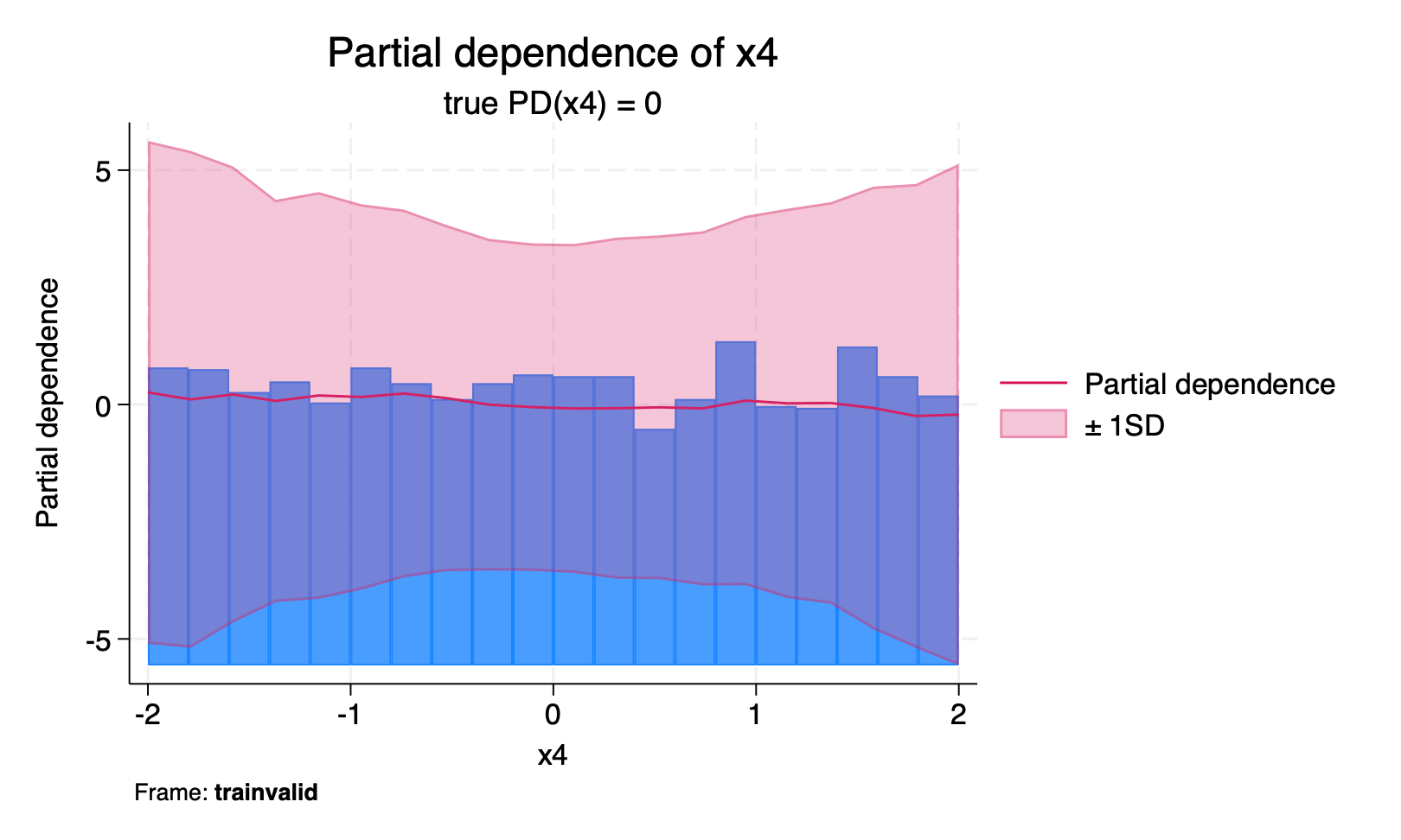
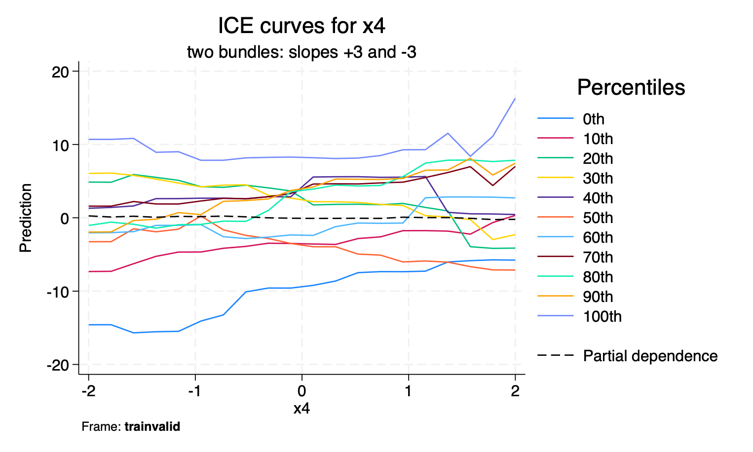
Figure 1: On the left, h2omlgraph pdp x4, sd. The curve is flat, which is the correct answer for the average effect. On the right, h2omlgraph ice x4 on the same model and the same frame. The individual curves separate into two groups with slopes near \(+3\) and \(-3\). Produced by figures.do.
The partial dependence plot is flat, which is expected, because the true average effect of \(x_4\) is zero in (2). A reader looking only at that plot would erroneously conclude that \(x_4\) does not matter. However, the effect of \(x_4\) is \(\pm 3\) per unit, among the largest in the model, and it averages to 0 only because the two subgroups cancel.
h2omlgraph ice reveals this immediately. This is the situation that individual conditional expectation plots were introduced to catch (Goldstein et al. 2015).
Note that no choice of frame would have provided a better partial dependence plot here. This is a limitation of averaging, not of the data used to average.
Permutation importance and the choice of frame
Recall that permutation importance shuffles a predictor and measures how much worse the predictions become. Now consider a model that has memorized its training data, including the noise. Shuffling a noise predictor will damage the memorized predictions, because the model was using that noise to identify individual training observations. On new data there is nothing to damage, because the noise never helped.
Molnar (2025) discusses this question at length and describes the case for both choices, noting that the argument is less consequential for a well-fitted model. Let us look at what happens with our overfit model.
We compare the training and testing frames on the same fitted model. On both frames, we hold samples(700), reps(10), and h2orseed(19) fixed, so neither frame is scored on more observations than the other, and we repeat this on 10 simulated datasets. The code is in permimp_frames.do.
Each cell of table 3 is a predictor's share of the total permutation importance within its own frame, averaged over the 10 datasets, and the last column counts the datasets in which the training share was the larger of the two.
Table 3: Permutation importance from h2omlgraph permimp with metric(mse), expressed as a percentage share of the within-frame total and averaged over 10 replications. The last column counts the replications in which the training frame share exceeded the testing-frame share. Produced by permimp_frames.do.
| Testing | Training | Difference | Training larger | |
|---|---|---|---|---|
| (%) | (%) | (pp) | ||
| \(x_1\), signal, no interaction | 31.18 | 35.97 | +4.79 | 10 of 10 |
| \(x_2\), signal, linear | 15.26 | 21.89 | +6.63 | 10 of 10 |
| \(x_4\), signal, interacting | 26.10 | 20.14 | -5.96 | 0 of 10 |
| \(g\), effect modifier | 25.54 | 14.39 | -11.15 | 0 of 10 |
| \(x_3\), correlated, no effect | 1.25 | 4.28 | +3.04 | 10 of 10 |
| \(x_5\), pure noise | 0.47 | 2.86 | +2.39 | 10 of 10 |
| \(x_6\), pure noise, binary | 0.20 | 0.46 | +0.26 | 9 of 10 |
The row to look at is \(x_5\) in table 3, which we constructed from random numbers and which has no relationship to \(y\) at all. It takes 2.86% of the training frame's importance and 0.47% of the testing frame's, a factor of about 6, at equal sample size, and it is larger on the training frame in every one of the 10 replications. Extra training observations would not fix this, which is the contrast with the partial dependence plot, where the number of observations accounted for the differences between frames.
The row for \(x_3\) in table 3 shows the same pattern and is the more common situation in practice. It also has no direct effect, being merely correlated with \(x_2\), and its share is 3.4 times larger on the training frame than on the testing frame.
The two rows that move the other way are \(x_4\) and \(g\), which are the two halves of the interaction term in (1). Both take a larger share on the testing frame in all 10 replications. We would not want to make conclusions based on only a single example, but it shows that the training frame does not inflate every predictor.
The comparison between \(x_5\) and \(x_6\) is also informative. Both are pure noise, and the only difference between them is that \(x_5\) is continuous and \(x_6\) is binary, yet \(x_5\) scores 6.2 times \(x_6\) on the training frame and 2.4 times on the testing frame. The tendency of tree-based importance measures to favor predictors with more possible split points is usually discussed in connection with impurity-based importance (Strobl et al. 2007), and here we can see it affecting permutation importance
as well.
Our suggestion for h2omlgraph permimp is to prefer the testing frame.
SHAP values and the choice of frame
The training frame was better for partial dependence and the testing frame for permutation importance, so where do SHAP values fall?
Loecher (2022) reports that SHAP values computed on training data can be biased in tree ensembles in a way related to the bias affecting impurity-based importance. To examine this, we compute a global measure of SHAP importance, the mean absolute SHAP value per predictor, from h2omlgraph shapsummary on each frame, over six replications. The code is in shap_frames.do. We report the absolute value of a SHAP before averaging, because a predictor can push one observation's prediction up and another's down. Each cell of table 4 is that average over the observations in the frame, and it measures how far a predictor typically moves an individual prediction.
Table 4: Mean absolute SHAP value by predictor and frame, averaged over six replications, using the same overfit model as before. Produced by shap_frames.do.
| Testing | Training | Ratio | Training larger | |||
|---|---|---|---|---|---|---|
| \(x_1\), signal, no interaction | 2.5094 | 2.5187 | 1.004 | 3 of 6 | ||
| \(x_2\), signal, linear | 1.6110 | 1.6186 | 1.005 | 4 of 6 | ||
| \(x_4\), signal, interacting | 0.7948 | 0.9759 | 1.229 | 6 of 6 | ||
| \(g\), effect modifier | 0.7561 | 0.7349 | 0.973 | 1 of 6 | ||
| \(x_3\), correlated, no effect | 0.2557 | 0.2841 | 1.113 | 5 of 6 | ||
| \(x_5\), pure noise | 0.1896 | 0.2256 | 1.192 | 6 of 6 | ||
| \(x_6\), pure noise, binary | 0.0679 | 0.0653 | 0.965 | 2 of 6 | ||
| Mean squared error | \(x_5\) importance share (%) | |||||
|---|---|---|---|---|---|---|
| Model | Training | Testing | Training | Testing | Difference | Training larger |
| (pp) | ||||||
| Overfit | 0.000 | 9.169 | 2.674 | 0.625 | 2.05 | 8 of 8 |
| Regularized | 4.089 | 5.464 | 0.432 | 0.091 | 0.34 | 8 of 8 |
| Tuned | 1.458 | 3.571 | 0.711 | 0.068 | 0.64 | 8 of 8 |
It can be seen that tuning shrinks the gap observed between the training and testing frames. The difference between the training and testing shares for \(x_5\) falls from 2.05 percentage points in the overfit model to 0.64 in the tuned one. In the tuned model, \(x_5\) takes 0.711% of the training frame's permutation importance and 0.068% of the testing frame's, against shares between 12% and 32% (computed in tuning_frames.do) for the 4 predictors that are important.
Thus, the frame changes the size of the numbers most when the model is poorly tuned. Once the model is well tuned, the frame no longer changes which predictors matter.
Limitations
All our results are based on a single simulated data-generating process, one model class, and one set of hyperparameter choices, so the results should be read as an illustration rather than as evidence about machine learning models in general.
Our data-generating process is deliberately simple, with one smooth nonlinearity, one linear term, and one two-way interaction, all with additive Gaussian noise. Real applications routinely involve higher-order interactions, non-Gaussian errors, and predictors whose distributions are far from uniform or normal. Heiß et al. (2026) run a broader simulation study across multiple data-generating processes and learners, and their conclusions should carry more weight than ours where the two differ.
We used gradient boosting only. Random forests, available through h2oml rfregress, average over trees differently and might well behave differently. In particular, for the results on the pure-noise predictors.
Our sample sizes are modest, at 4,000 observations before splitting. Because several of the effects we report scale with sample size, the balance between bias and variance would shift in a larger dataset.
We examined regression with a continuous response. Classification introduces a choice of metric, and permutation importance in particular can rank predictors differently depending on whether metric(auc) or metric(logloss) is used, because importance is always defined relative to a loss.
Finally, our replication counts are small, between 6 and 15 depending on the experiment, which is enough to establish the direction of the effects we report but not to pin down their magnitudes precisely. Where we report counts such as eight of eight, those describe our replications and not a formal test.
We should also be clear about what none of these methods can do. All the commands discussed here describe an fitted model. They do not identify causal effects, and a partial dependence curve should not be read as the effect of intervening on a predictor unless separate assumptions are met (Molnar 2025). When predictors are correlated, as \(x_2\) and \(x_3\) are in our simulation, partial dependence evaluates the model at combinations of values that may never occur in the data, which is a well-known issue (Apley and Zhu 2020; Hooker et al. 2021).
Recommendations
With those limitations in mind, table 6 summarizes our recommendations.
Table 6: Recommended frame choices based on the example in this post
| Command | Recommended frame | Reasoning |
|---|---|---|
| pdp, ice | The frame with the most observations | These curves are averages, so their error is dominated by estimation variance, which decreases as observations are added. Reusing training observations introduces a bias in principle, but we found it too small to outweigh the larger sample. The choice of a frame matters most for predictors that interact with others. |
| permimp | Testing, or another frame the model has not seen | Importance is measured by how much the loss increases when a predictor is permuted, so it reflects what the model has memorized as well as what it has learned. A predictor fit to noise looks important on the data the model was fit on. Only holdout observations separate the two, and a larger frame will not. |
| shapsummary, shapvalues | The frame holding the observations you want to explain | SHAP values decompose predictions the model has already made, so the frame decides which observations are described rather than how accurate the description is. Changing it will not correct a model that uses a predictor it should not. |
| varimp | Training, and there is no option to change it | Impurity-based importance is accumulated as the trees are grown, so it can describe only the data the model was fit on. It also favors predictors offering more split points (Strobl et al. 2007), so use it as a description of how the trees were built. |
Apley, D. W., and J. Zhu. 2020. Visualizing the effects of predictor variables in black box supervised learning models. Journal of the Royal Statistical Society, B ser., 82: 1059–1086. https://doi.org/10.1111/rssb.12377.
Breiman, L. 2001. Random forests. Machine Learning 45: 5–32. https://doi.org/10.1023/A:1010933404324.
Friedman, J. H. 2001. Greedy function approximation: A gradient boosting machine. Annals of Statistics 29: 1189–1232. https://doi.org/10.1214/aos/1013203451.
Goldstein, A., A. Kapelner, J. Bleich, and E. Pitkin. 2015. Peeking inside the black box: Visualizing statistical learning with plots of individual conditional expectation. Journal of Computational and Graphical Statistics 24: 44--65. https://doi.org/10.1080/10618600.2014.907095.
Heiß, T., C. Bögel, B. Bischl, and G. Casalicchio. 2026. Analyzing error sources in global feature effect estimation. arXiv:2603.15057 [stat.ML]. https://doi.org/10.48550/arXiv.2603.15057.
Hooker, G., L. Mentch, and S. Zhou. 2021. Unrestricted permutation forces extrapolation: Variable importance requires at least one more model. Statistics and Computing 31: 82. https://doi.org/10.1007/s11222-021-10057-z.
Loecher, M. 2022. "Debiasing MDI feature importance and SHAP values in tree ensembles". In Machine Learning and Knowledge Extraction, edited by A. Holzinger, P. Kieseberg, A. M. Tjoa, and E. Weippl, vol. 13480: 114–129. Cham: Springer. https://doi.org/10.1007/978-3-031-14463-9_8.
Lundberg, S. M., and S.-I. Lee. 2017. "A unified approach to interpreting model predictions". In Advances in Neural Information Processing Systems, edited by U. von Luxburg, I. Guyon, S. Bengio, H. Wallach, and R. Fergus, vol. 30: 4765–4774. Red Hook, NY: Curran Associates.
Lundberg, S. M., G. Erion, H. Chen, A. DeGrave, J. M. Prutkin, B. Nair, R. Katz, J. Himmelfarb, N. Bansal, and S.-I. Lee. 2020. From local explanations to global understanding with explainable AI for trees. Nature Machine Intelligence 2: 56–67. https://doi.org/10.1038/s42256-019-0138-9.
Molnar, C. 2025. Interpretable Machine Learning: A Guide for Making Black Box Models Explainable. 3rd ed. https://christophm.github.io/interpretable-ml-book/.
Strobl, C., A.-L. Boulesteix, A. Zeileis, and T. Hothorn. 2007. Bias in random forest variable importance measures: Illustrations, sources and a solution. BMC Bioinformatics 8: 25. https://doi.org/10.1186/1471-2105-8-25.