I want to show you a way of picturing and thinking about matrices. The topic for today is the square matrix, which we will call A. I’m going to show you a way of graphing square matrices, although we will have to limit ourselves to the 2 x 2 case. That will be, as they say, without loss of generality. The technique I’m about to show you could be used with 3 x 3 matrices if you had a better 3-dimensional monitor, and as will be revealed, it could be used on 3 x 2 and 2 x 3 matrices, too. If you had more imagination, we could use the technique on 4 x 4, 5 x 5, and even higher-dimensional matrices.

But we will limit ourselves to 2 x 2. A might be

From now on, I’ll write matrices as

A = (2, 1 \ 1.5, 2)

where commas are used to separate elements on the same row and backslashes are used to separate the rows.

To graph A, I want you to think about

y = Ax

where

y: 2 x 1,

A: 2 x 2, and

x: 2 x 1.

That is, we are going to think about A in terms of its effect in transforming points in space from x to y. For instance, if we had the point

x = (0.75 \ 0.25)

then

y = (1.75 \ 1.625)

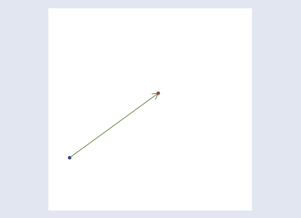
because by the rules of matrix multiplication y[1] = 0.75*2 + 0.25*1 = 1.75 and y[2] = 0.75*1.5 + 0.25*2 = 1.625. The matrix A transforms the point (0.75 \ 0.25) to (1.75 \ 1.625). We could graph that:

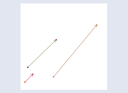
To get a better understanding of how A transforms the space, we could graph additional points:

I do not want you to get lost among the individual points which A could transform, however. To focus better on A, we are going to graph y = Ax for all x. To do that, I’m first going to take a grid,

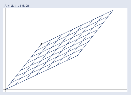
One at a time, I’m going to take every point on the grid, call the point x, and run it through the transform y = Ax. Then I’m going to graph the transformed points:

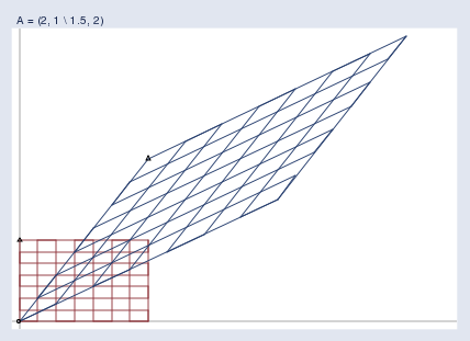
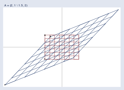
Finally, I’m going to superimpose the two graphs:

In this way, I can now see exactly what A = (2, 1 \ 1.5, 2) does. It stretches the space, and skews it.

I want you to think about transforms like A as transforms of the space, not of the individual points. I used a grid above, but I could just as well have used a picture of the Eiffel tower and, pixel by pixel, transformed it by using y = Ax. The result would be a distorted version of the original image, just as the the grid above is a distorted version of the original grid. The distorted image might not be helpful in understanding the Eiffel Tower, but it is helpful in understanding the properties of A. So it is with the grids.

Notice that in the above image there are two small triangles and two small circles. I put a triangle and circle at the bottom left and top left of the original grid, and then again at the corresponding points on the transformed grid. They are there to help you orient the transformed grid relative to the original. They wouldn’t be necessary had I transformed a picture of the Eiffel tower.

I’ve suppressed the scale information in the graph, but the axes make it obvious that we are looking at the first quadrant in the graph above. I could just as well have transformed a wider area.

Regardless of the region graphed, you are supposed to imagine two infinite planes. I will graph the region that makes it easiest to see the point I wish to make, but you must remember that whatever I’m showing you applies to the entire space.

We need first to become familiar with pictures like this, so let’s see some examples. Pure stretching looks like this:

Pure compression looks like this:

Pay attention to the color of the grids. The original grid, I’m showing in red; the transformed grid is shown in blue.

A pure rotation (and stretching) looks like this:

Note the location of the triangle; this space was rotated around the origin.

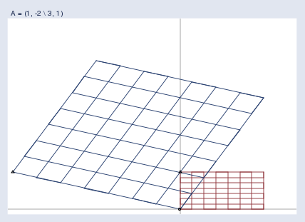
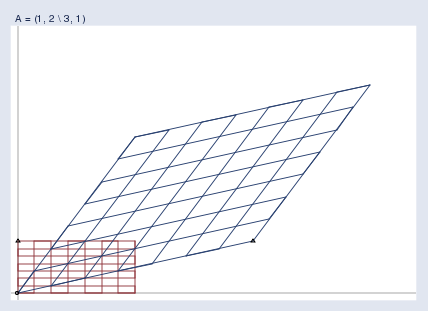
Here’s an interesting matrix that produces a surprising result: A = (1, 2 \ 3, 1).

This matrix flips the space! Notice the little triangles. In the original grid, the triangle is located at the top left. In the transformed space, the corresponding triangle ends up at the bottom right! A = (1, 2 \ 3, 1) appears to be an innocuous matrix — it does not even have a negative number in it — and yet somehow, it twisted the space horribly.

So now you know what 2 x 2 matrices do. They skew,stretch, compress, rotate, and even flip 2-space. In a like manner, 3 x 3 matrices do the same to 3-space; 4 x 4 matrices, to 4-space; and so on.

Well, you are no doubt thinking, this is all very entertaining. Not really useful, but entertaining.

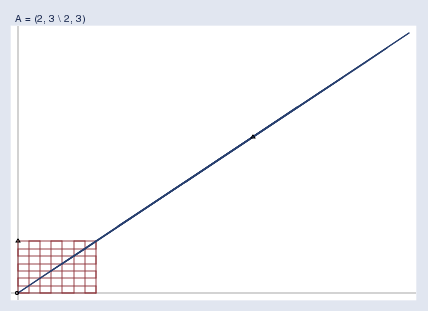
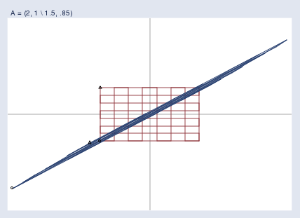
Okay, tell me what it means for a matrix to be singular. Better yet, I’ll tell you. It means this:

A singular matrix A compresses the space so much that the poor space is squished until it is nothing more than a line. It is because the space is so squished after transformation by y = Ax that one cannot take the resulting y and get back the original x. Several different x values get squished into that same value of y. Actually, an infinite number do, and we don’t know which you started with.

A = (2, 3 \ 2, 3) squished the space down to a line. The matrix A = (0, 0 \ 0, 0) would squish the space down to a point, namely (0 0). In higher dimensions, say, k, singular matrices can squish space into k-1, k-2, …, or 0 dimensions. The number of dimensions is called the rank of the matrix.

Singular matrices are an extreme case of nearly singular matrices, which are the bane of my existence here at StataCorp. Here is what it means for a matrix to be nearly singular:

Nearly singular matrices result in spaces that are heavily but not fully compressed. In nearly singular matrices, the mapping from x to y is still one-to-one, but x‘s that are far away from each other can end up having nearly equal y values. Nearly singular matrices cause finite-precision computers difficulty. Calculating y = Ax is easy enough, but to calculate the reverse transform x = A^-1y means taking small differences and blowing them back up, which can be a numeric disaster in the making.

So much for the pictures illustrating that matrices transform and distort space; the message is that they do. This way of thinking can provide intuition and even deep insights. Here’s one:

In the above graph of the fully singular matrix, I chose a matrix that not only squished the space but also skewed the space some. I didn’t have to include the skew. Had I chosen matrix A = (1, 0 \ 0, 0), I could have compressed the space down onto the horizontal axis. And with that, we have a picture of nonsquare matrices. I didn’t really need a 2 x 2 matrix to map 2-space onto one of its axes; a 2 x 1 vector would have been sufficient. The implication is that, in a very deep sense, nonsquare matrices are identical to square matrices with zero rows or columns added to make them square. You might remember that; it will serve you well.

Here’s another insight:

In the linear regression formula b = (X‘X)^-1X‘y, (X‘X)^-1 is a square matrix, so we can think of it as transforming space. Let’s try to understand it that way.

Begin by imagining a case where it just turns out that (X‘X)^-1 = I. In such a case, (X‘X)^-1 would have off-diagonal elements equal to zero, and diagonal elements all equal to one. The off-diagonal elements being equal to 0 means that the variables in the data are uncorrelated; the diagonal elements all being equal to 1 means that the sum of each squared variable would equal 1. That would be true if the variables each had mean 0 and variance 1/N. Such data may not be common, but I can imagine them.

If I had data like that, my formula for calculating b would be b = (X‘X)^-1X‘y = IX‘y = X‘y. When I first realized that, it surprised me because I would have expected the formula to be something like b = X^-1y. I expected that because we are finding a solution to y = Xb, and b = X^-1y is an obvious solution. In fact, that’s just what we got, because it turns out that X^-1y = X‘y when (X‘X)^-1 = I. They are equal because (X‘X)^-1 = I means that X‘X = I, which means that X‘ = X^-1. For this math to work out, we need a suitable definition of inverse for nonsquare matrices. But they do exist, and in fact, everything you need to work it out is right there in front of you.

Anyway, when correlations are zero and variables are appropriately normalized, the linear regression calculation formula reduces to b = X‘y. That makes sense to me (now) and yet, it is still a very neat formula. It takes something that is N x k — the data — and makes k coefficients out of it. X‘y is the heart of the linear regression formula.

Let’s call b = X‘y the naive formula because it is justified only under the assumption that (X‘X)^-1 = I, and real X‘X inverses are not equal to I. (X‘X)^-1 is a square matrix and, as we have seen, that means it can be interpreted as compressing, expanding, and rotating space. (And even flipping space, although it turns out the positive-definite restriction on X‘X rules out the flip.) In the formula (X‘X)^-1X‘y, (X‘X)^-1 is compressing, expanding, and skewing X‘y, the naive regression coefficients. Thus (X‘X)^-1 is the corrective lens that translates the naive coefficients into the coefficient we seek. And that means X‘X is the distortion caused by scale of the data and correlations of variables.

Thus I am entitled to describe linear regression as follows: I have data (y, X) to which I want to fit y = Xb. The naive calculation is b = X‘y, which ignores the scale and correlations of the variables. The distortion caused by the scale and correlations of the variables is X‘X. To correct for the distortion, I map the naive coefficients through (X‘X)^-1.

Intuition, like beauty, is in the eye of the beholder. When I learned that the variance matrix of the estimated coefficients was equal to s²(X‘X)^-1, I immediately thought: s² — there’s the statistics. That single statistical value is then parceled out through the corrective lens that accounts for scale and correlation. If I had data that didn’t need correcting, then the standard errors of all the coefficients would be the same and would be identical to the variance of the residuals.

If you go through the derivation of s²(X‘X)^-1, there’s a temptation to think that s² is merely something factored out from the variance matrix, probably to emphasize the connection between the variance of the residuals and standard errors. One easily loses sight of the fact that s² is the heart of the matter, just as X‘y is the heart of (X‘X)^-1X‘y. Obviously, one needs to view both s² and X‘y though the same corrective lens.

I have more to say about this way of thinking about matrices. Look for part 2 in the near future. Update: part 2 of this posting, “Understanding matrices intuitively, part 2, eigenvalues and eigenvectors”, may now be found at http://blog.stata.com/2011/03/09/understanding-matrices-intuitively-part-2/.