Teach statistical concepts with Stata
My first statistics course primarily consisted of plugging numbers into formulas. I did not leave that course with any real idea of how statistics differed from basic algebra. The next course I took is what put it all together, and I’ve loved statistics ever since. In that course, we examined the relationships between a population and its samples. I learned that using just a small amount of data, statistics enables us to make inferences about the entire population. Now that is cool!
In this blog, I provide tools for introductory statistics course instructors to demonstrate the concepts of sampling distributions, standard errors, confidence intervals (CIs), and p-values. To illustrate these concepts, we’ll use the following research question:
Do residents of College Station, TX (CSTX), who have been diagnosed with diabetes have a higher average body mass index (BMI) than CSTX residents without a diabetes diagnosis?
The population
If you have a dataset to use as a population—wonderful! Use that. Or you can have your students collect data, for example, from every 11th grader. Otherwise, you’ll need to simulate a population dataset. I have no means to collect data from everyone in CSTX, so I will demonstrate using a simulated population.
First, I create a new data frame called population and change into it.
. frame create population
. frame change population
I set a random-number seed to ensure reproducibility and set the number of observations. I’m using 135,000 because that’s the estimated number of residents in CSTX, my population.
. set seed 12
. set obs 135000
Number of observations (_N) was 0, now 135,000.
Then we will use Stata’s random-number generators to simulate BMI and diabetes incidence in the population. See [FN] Random-number functions, or type help random number functions into Stata’s Command window for a full list of available distributions.
We will use a normal distribution for BMI and a binomial distribution for diabetes. I do a quick internet search to get hyperparameters for these distributions, that is, the mean and standard deviation of BMI in the US population and the proportion with a diabetes diagnosis. The number of events in the binomial distribution is 1 because we are simulating only one event: diabetes. I add 2 to everyone in the diabetes group so that their average BMI is 2 higher than the nondiabetic group.
. generate diabetes = rbinomial(1,0.12)
. generate bmi = rnormal(27,6) + 2 * diabetes
It’s good practice to assign labels and value labels (if applicable) to generated variables. Let’s do
that now.
. label variable bmi "Body mass index"
. label variable diabetes "Diabetes diagnosis"
. label define diab 0 "Not diabetic" 1 "Diabetic"
. label values diabetes diab
Samples
We can extract a single sample from this population using the sample command. We’ll sample just 0.1% of the population. We first use preserve to preserve our population.
. preserve
. sample 0.1
(134,865 observations deleted)
Let’s conduct a t test on this sample to test whether the mean BMI differs by diabetes group.
. ttest bmi, by(diabetes)

Two-sample t test with equal variances
------------------------------------------------------------------------------
   Group |     Obs        Mean    Std. err.   Std. dev.   [95% conf. interval]
---------+--------------------------------------------------------------------
Not diab |     114    28.31035    .5315609    5.675517    27.25723    29.36347
Diabetic |      21    29.49885      .91868    4.209921    27.58252    31.41518
---------+--------------------------------------------------------------------
Combined |     135    28.49523    .4713703    5.476828    27.56294    29.42752
---------+--------------------------------------------------------------------
    diff |           -1.188497    1.301377                -3.76257    1.385575
------------------------------------------------------------------------------
    diff = mean(Not diab) - mean(Diabetic)                        t =  -0.9133
H0: diff = 0                                     Degrees of freedom =      133

    Ha: diff < 0                 Ha: diff != 0                 Ha: diff > 0
 Pr(T < t) = 0.1814         Pr(|T| > |t|) = 0.3628          Pr(T > t) = 0.8186
The first two sections give some information about each group and their combined sample. The last row, labeled diff, is what we are testing. The difference in means in BMI in this sample is 1.19 (SE = 1.30; 95% CI [-3.76, 1.39]). The difference in means estimate in the results table is negative because it subtracts the diabetic mean BMI from the nondiabetic mean BMI.
The t statistic is just the difference in means divided by its standard error. We can calculate this manually by using the difference in means and standard error in the returned results.
. return list

scalars:
            r(ub_diff) =  1.385575269027033
            r(lb_diff) =  -3.762570056926808
            r(mu_diff) =  -1.188497393949888
        r(ub_combined) =  29.42751874623384
        r(lb_combined) =  27.56294203811313
        r(se_combined) =  .4713703167472302
        r(mu_combined) =  28.49523039217349
         r(N_combined) =  135
               r(ub_2) =  31.41518328412929
               r(lb_2) =  27.58251754333305
               r(se_2) =  .9186799859364339
               r(ub_1) =  29.36347104716379
               r(lb_1) =  27.25723499239878
               r(se_1) =  .5315609062940896
              r(level) =  95
                 r(sd) =  5.476828159975613
               r(sd_2) =  4.209920574994674
               r(sd_1) =  5.675517392222678
                 r(se) =  1.301376679922003
                r(p_u) =  .8186212430198624
                r(p_l) =  .1813787569801376
                  r(p) =  .3627575139602752
                  r(t) =  -.9132616346107564
               r(df_t) =  133
               r(mu_2) =  29.49885041373117
                r(N_2) =  21
               r(mu_1) =  28.31035301978128
                r(N_1) =  114
We use the difference in means, saved as r(mu_diff), and the standard error, saved as r(se), to calculate t.
. display r(mu_diff)/r(se)
-.91326163
This is the same t statistic reported under the results table. If you’re ever unsure how a statistic is being calculated, visit the Methods and formulas in [R] ttest. Using this sample, we don’t have enough evidence to conclude that there is a difference between groups, t(133) = 0.91, p = 0.181. We use the lower-tail p-value because our hypothesis is that the diabetic group had a higher mean BMI than the nondiabetic group.
What if we had sampled a different set of observations? First, let’s restore and then preserve our population again.
. restore
. preserve
Now, let’s use a different random-number seed, then sample and test again.
. set seed 78

. sample 0.1
(134,865 observations deleted)

. ttest bmi, by(diabetes)

Two-sample t test with equal variances
------------------------------------------------------------------------------
   Group |     Obs        Mean    Std. err.   Std. dev.   [95% conf. interval]
---------+--------------------------------------------------------------------
Not diab |     119    27.38515    .5024667    5.481265    26.39013    28.38017
Diabetic |      16    30.22711    1.023486    4.093946     28.0456    32.40862
---------+--------------------------------------------------------------------
Combined |     135    27.72197    .4649424    5.402142     26.8024    28.64155
---------+--------------------------------------------------------------------
    diff |           -2.841961    1.422678               -5.655963   -.0279588
------------------------------------------------------------------------------
    diff = mean(Not diab) - mean(Diabetic)                        t =  -1.9976
H0: diff = 0                                     Degrees of freedom =      133

    Ha: diff < 0                 Ha: diff != 0                 Ha: diff > 0
 Pr(T < t) = 0.0239         Pr(|T| > |t|) = 0.0478          Pr(T > t) = 0.9761
Using this sample, we have evidence that there is a group difference in mean BMI, t(133) = 2.00, p = 0.024.
Let’s put this sample into a frame called sample, then restore our population.
. frame put *, into(sample)
. restore
Sample-to-sample variability is key to being able to make statistical inferences. Because we have the population, we can build a sampling distribution to see this variability firsthand.
The sampling distribution
We start by creating a new data frame named sampling with variables diff, se, ub, and lb.
. frame create sampling diff se ub lb
Then we use a for loop to collect 100 samples, each containing 0.1% of the population. We conduct t tests on each of these samples and post the estimated difference in means, standard error, and upper and lower bounds of the CI to the sampling frame. We add quietly in front of sample and ttest to suppress their outputs.
. forvalues i = 1/100 {
  2. preserve
  3. quietly sample 0.1
  4. quietly ttest bmi, by(diabetes)
  5. frame post sampling (r(mu_diff)) (r(se)) (r(ub_diff)) (r(lb_diff))
  6. restore
  7. }
We change to the sampling frame we just created.
. frame change sampling
Let’s begin by looking at a histogram of the difference in means.
. histogram diff
(bin=10, start=-6.039753, width=.72761365)
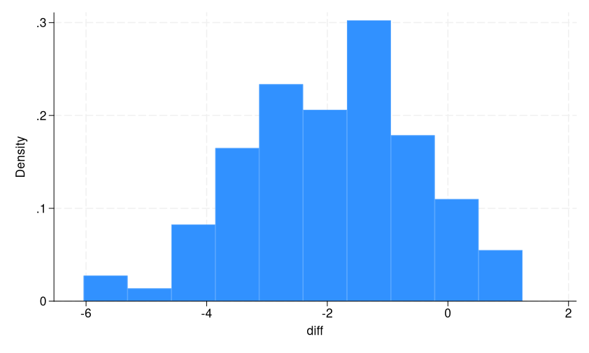
This is a sampling distribution of the difference in means in BMI by diabetes diagnosis. We can see that most of our samples are around -2, as expected, but there is a substantial spread. Also note that it is approximately normally distributed. This is due to the central limit theorem, which states that the distribution of sample means of independent, identically distributed random variables approaches a normal distribution as the sample size increases, regardless of the original population’s distribution. (Having students start with other population distributions can be a fun exercise!)
Standard error
The standard deviation of the sampling distribution is called the standard error. When we conduct a t test on a sample, we also get an estimate of the standard error. It tells us about the expected distance between our sample estimate and the population parameter.
. summarize se diff

    Variable |        Obs        Mean    Std. dev.       Min        Max
-------------+---------------------------------------------------------
          se |        100    1.610917    .2193768   1.206266   2.400811
        diff |        100   -1.956383    1.477907  -6.039753   1.236384
The estimated standard error according to this sampling distribution is 1.48. We see that the average estimated standard error from the samples, 1.61, is close to this number, even with only 100 samples. As the number of samples in our sampling distribution increases, these two numbers will converge, and the difference in means will approach -2.
You can also have your students use different sample sizes when building a sampling distribution to see how this impacts the standard error. Use the count option of the sample command to directly sample a specific number of observations rather than a percentage.
CI
The CI is another way of thinking about the variability across samples. If we repeat the sampling process many times, 95% of the 95% CIs constructed will contain the true, unknown population parameter. Because we have 100 samples in our sampling distribution, we expect 95 of them to contain -2, the true difference.
Let’s look at the CIs we collected from each of the samples in our sampling distribution.
We sort, then create variable i to order them on the x axis from smallest to largest point estimate, and then use twoway rpcap to visualize them.
. sort diff
. generate i = _n
. twoway (rpcap lb ub diff i)
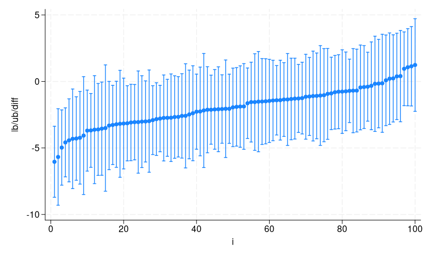
Let’s add a reference line at the true difference, -2, and add titles.
. twoway (rpcap lb ub diff i), ytitle("Difference in means") yline(-2)
> xtitle("") xlabel(none, nolabels) title("100 95% confidence intervals")
> subtitle("95 contain the true population parameter (dashed line)")
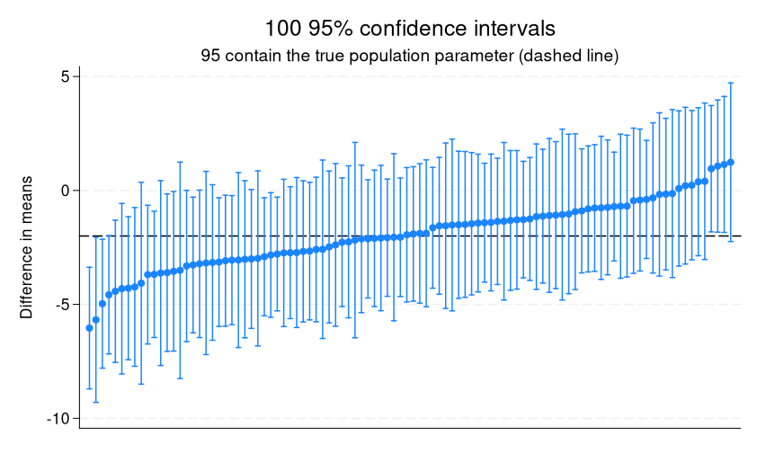
We can see that the first CI and the last four CIs don’t contain the true value.
When we calculate a CI in a sample, it is the estimated range of values within which we are 95% confident the true population parameter lies. With this demonstration, we can easily see that “95% confident” refers to the percentage of intervals containing the true parameter across repeated samples rather than the often incorrectly used interpretation that there is a 95% chance (or 0.95 probability) that the true parameter lies within the interval constructed from a single sample.
p-values
There is one more concept I would like to cover: p-values. They are infamously misunderstood and misused. Thus, I think it’s important that students understand what they are and what they really tell us.
To understand p-values will require building a null sampling distribution, that is, a sampling distribution from a population in which there is no effect. To create a null sampling distribution, we can follow the same process we used for the alternative sampling distribution without adding 2 to the diabetes group, but we don’t have to. We know exactly what the distribution of t statistics will look like from a null population; they will be t distributed! That’s why we bother with creating test statistics in the first place.
Let’s first visualize a t distribution using a twoway function graph.
. twoway (function density = tden(133,x), range(-3 3)), xtitle({it:t})
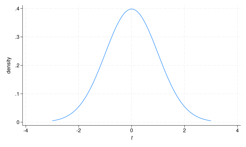
This is the sampling distribution of t values we would expect from a population in which there is no difference in mean BMI between diabetics and nondiabetics. As expected, it centers around 0.
Let’s see the t test on our last sample once more.
. frame sample: ttest bmi, by(diabetes)

Two-sample t test with equal variances
------------------------------------------------------------------------------
   Group |     Obs        Mean    Std. err.   Std. dev.   [95% conf. interval]
---------+--------------------------------------------------------------------
Not diab |     119    27.38515    .5024667    5.481265    26.39013    28.38017
Diabetic |      16    30.22711    1.023486    4.093946     28.0456    32.40862
---------+--------------------------------------------------------------------
Combined |     135    27.72197    .4649424    5.402142     26.8024    28.64155
---------+--------------------------------------------------------------------
    diff |           -2.841961    1.422678               -5.655963   -.0279588
------------------------------------------------------------------------------
    diff = mean(Not diab) - mean(Diabetic)                        t =  -1.9976
H0: diff = 0                                     Degrees of freedom =      133

    Ha: diff < 0                 Ha: diff != 0                 Ha: diff > 0
 Pr(T < t) = 0.0239         Pr(|T| > |t|) = 0.0478          Pr(T > t) = 0.9761
We get a t statistic of -1.99, and at the bottom we see three p-values: lower-, two-, and upper-tailed.
The lower-tailed p-value tells us that if there were no difference in means in BMI in the population, the probability of calculating a t statistic that is less than -1.99 is 0.024, or about 2%. We can replicate this number using the cumulative Student’s t distribution function, t(df, t), where df is the degrees of freedom from our sample, 133, and t is the t statistic from our sample, -1.9976.
. display t(133,- 1.9976)
.02390008
This function calculates the cumulative probability of the t distribution up to -1.9976. To visualize this, we add an x line to our t distribution graph.
. twoway (function density = tden(133,x), range(-3 3)),
> xtitle({it:t}) xline(-2)
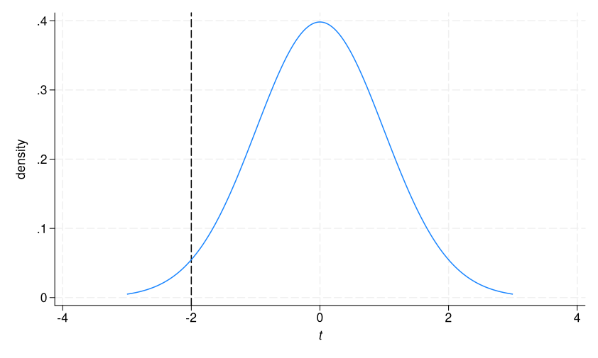
2.4% of the distribution is to the left of the dashed line.
The upper-tailed p-value tells us that if there were no difference in means in BMI in the population, the probability of calculating a t statistic greater than -1.99 is 0.976, or about 98%. Again, we can replicate this number using the cumulative distribution function, this time subtracting from 1.
. display 1 - t(133,- 1.9976)
.97609992
Now we are calculating the probability to the right of the dashed line in our graph, which is 1 – the probability to the left.
The two-tailed p-value is simply twice the lower-valued p-value, in this case the lower-tailed.
. display 2 * t(133,- 1.9976)
.04780016
It tells us the probability of calculating a t statistic less than -1.99 or greater than 1.99. We can add a second line to our graph to visualize this.
. twoway (function density = tden(133,x), range(-3 3)), xtitle({it:t})
> xline(-2) xline(2)
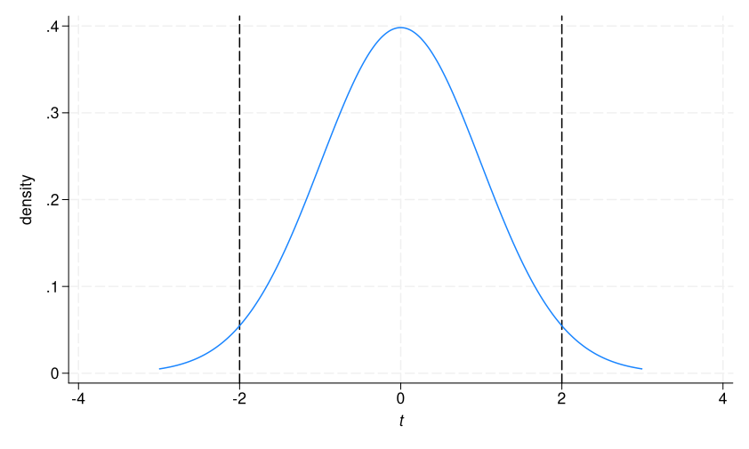
The two-tailed p-value is the proportion to the left of the first dashed line plus the proportion to the right of the second dashed line. In other words, it is telling us that, if there is no true difference between groups, there is 5% probability of getting a t statistic as or more extreme than the statistic we calculated in this sample.
Conclusion
In this blog, we have explored how to demonstrate the following core pillars of statistical inference through simulation and visualization: sampling distributions, standard errors, CIs, and p-values.
Statistics becomes compelling for students when they can see the relationships between a population and its samples for themselves. To bring these demonstrations into your classroom and help your students learn much faster, you can download the do-file here.