Last time, I showed you a way to graph and to think about matrices. This time, I want to apply the technique to eigenvalues and eigenvectors. The point is to give you a picture that will guide your intuition, just as it was previously.

Before I go on, several people asked after reading part 1 for the code I used to generate the graphs. Here it is, both for part 1 and part 2: matrixcode.zip.

The eigenvectors and eigenvalues of matrix A are defined to be the nonzero x and λ values that solve

Ax = λx

I wrote a lot about Ax in the last post. Just as previously, x is a point in the original, untransformed space and Ax is its transformed value. λ on the right-hand side is a scalar.

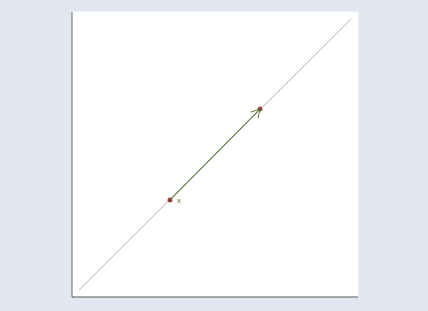
Multiplying a point by a scalar moves the point along a line that passes through the origin and the point:

The figure above illustrates y=λx when λ>1. If λ were less than 1, the point would move toward the origin and if λ were also less than 0, the point would pass right by the origin to land on the other side. For any point x, y=λx will be somewhere on the line passing through the origin and x.

Thus Ax = λx means the transformed value Ax lies on a line passing through the origin and the original x. Points that meet that restriction are eigenvectors (or more correctly, as we will see, eigenpoints, a term I just coined), and the corresponding eigenvalues are the λ‘s that record how far the points move along the line.

Actually, if x is a solution to Ax = λx, then so is every other point on the line through 0 and x. That’s easy to see. Assume x is a solution to Ax = λx and substitute cx for x: Acx = λcx. Thus x is not the eigenvector but is merely a point along the eigenvector.

And with that prelude, we are now in a position to interpret Ax = λx fully. Ax = λx finds the lines such that every point on the line, say, x, transformed by Ax moves to being another point on the same line. These lines are thus the natural axes of the transform defined by A.

The equation Ax = λx and the instructions “solve for nonzero x and λ” are deceptive. A more honest way to present the problem would be to transform the equation to polar coordinates. We would have said to find θ and λ such that any point on the line (r, θ) is transformed to (λr, θ). Nonetheless, Ax = λx is how the problem is commonly written.

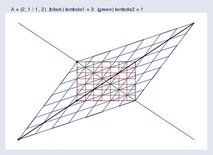
However we state the problem, here is the picture and solution for A = (2, 1 \ 1, 2)

I used Mata’s eigensystem() function to obtain the eigenvectors and eigenvalues. In the graph, the black and green lines are the eigenvectors.

The first eigenvector is plotted in black. The “eigenvector” I got back from Mata was (0.707 \ 0.707), but that’s just one point on the eigenvector line, the slope of which is 0.707/0.707 = 1, so I graphed the line y = x. The eigenvalue reported by Mata was 3. Thus every point x along the black line moves to three times its distance from the origin when transformed by Ax. I suppressed the origin in the figure, but you can spot it because it is where the black and green lines intersect.

The second eigenvector is plotted in green. The second “eigenvector” I got back from Mata was (-0.707 \ 0.707), so the slope of the eigenvector line is 0.707/(-0.707) = -1. I plotted the line y = –x. The eigenvalue is 1, so the points along the green line do not move at all when transformed by Ax; y=λx and λ=1.

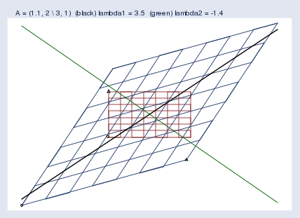
Here’s another example, this time for the matrix A = (1.1, 2 \ 3, 1):

The first “eigenvector” and eigenvalue Mata reported were… Wait! I’m getting tired of quoting the word eigenvector. I’m quoting it because computer software and the mathematical literature call it the eigenvector even though it is just a point along the eigenvector. Actually, what’s being described is not even a vector. A better word would be eigenaxis. Since this posting is pedagogical, I’m going to refer to the computer-reported eigenvector as an eigenpoint along the eigenaxis. When you return to the real world, remember to use the word eigenvector.

The first eigenpoint and eigenvalue that Mata reported were (0.640 \ 0.768) and λ = 3.45. Thus the slope of the eigenaxis is 0.768/0.640 = 1.2, and points along that line — the green line — move to 3.45 times their distance from the origin.

The second eigenpoint and eigenvalue Mata reported were (-0.625 \ 0.781) and λ = -1.4. Thus the slope is -0.781/0.625 = -1.25, and points along that line move to -1.4 times their distance from the origin, which is to say they flip sides and then move out, too. We saw this flipping in my previous posting. You may remember that I put a small circle and triangle at the bottom left and bottom right of the original grid and then let the symbols be transformed by A along with the rest of space. We saw an example like this one, where the triangle moved from the top-left of the original space to the bottom-right of the transformed space. The space was flipped in one of its dimensions. Eigenvalues save us from having to look at pictures with circles and triangles; when a dimension of the space flips, the corresponding eigenvalue is negative.

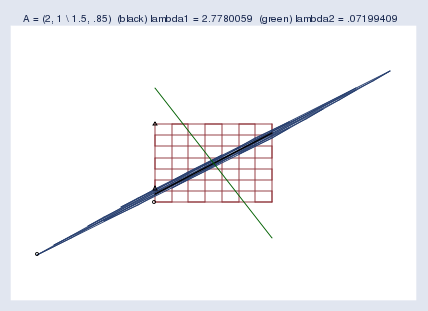
We examined near singularity last time. Let’s look again, and this time add the eigenaxes:

The blue blob going from bottom-left to top-right is both the compressed space and the first eigenaxis. The second eigenaxis is shown in green.

Mata reported the first eigenpoint as (0.789 \ 0.614) and the second as (-0.460 \ 0.888). Corresponding eigenvalues were reported as 2.78 and 0.07. I should mention that zero eigenvalues indicate singular matrices and small eigenvalues indicate nearly singular matrices. Actually, eigenvalues also reflect the scale of the matrix. A matrix that compresses the space will have all of its eigenvalues be small, and that is not an indication of near singularity. To detect near singularity, one should look at the ratio of the largest to the smallest eigenvalue, which in this case is 0.07/2.78 = 0.03.

Despite appearances, computers do not find 0.03 to be small and thus do not think of this matrix as being nearly singular. This matrix gives computers no problem; Mata can calculate the inverse of this without losing even one binary digit. I mention this and show you the picture so that you will have a better appreciation of just how squished the space can become before computers start complaining.

When do well-programmed computers complain? Say you have a matrix A and make the above graph, but you make it really big — 3 miles by 3 miles. Lay your graph out on the ground and hike out to the middle of it. Now get down on your knees and get out your ruler. Measure the spread of the compressed space at its widest part. Is it an inch? That’s not a problem. One inch is roughly 5*10^-6 of the original space (that is, 1 inch by 3 miles wide). If that were a problem, users would complain. It is not problematic until we get around 10^-8 of the original area. Figure about 0.002 inches.

There’s more I could say about eigenvalues and eigenvectors. I could mention that rotation matrices have no eigenvectors and eigenvalues, or at least no real ones. A rotation matrix rotates the space, and thus there are no transformed points that are along their original line through the origin. I could mention that one can rebuild the original matrix from its eigenvectors and eigenvalues, and from that, one can generalize powers to matrix powers. It turns out that A^-1 has the same eigenvectors as A; its eigenvalues are λ^-1 of the original’s. Matrix AA also has the same eigenvectors as A; its eigenvalues are λ². Ergo, A^p can be formed by transforming the eigenvalues, and it turns out that, indeed, A^½ really does, when multiplied by itself, produce A.