How to simulate multilevel/longitudinal data
I was recently talking with my friend Rebecca about simulating multilevel data, and she asked me if I would show her some examples. It occurred to me that many of you might also like to see some examples, so I decided to post them to the Stata Blog.
Introduction
We simulate data all the time at StataCorp and for a variety of reasons.
One reason is that real datasets that include the features we would like are often difficult to find. We prefer to use real datasets in the manual examples, but sometimes that isn’t feasible and so we create simulated datasets.
We also simulate data to check the coverage probabilities of new estimators in Stata. Sometimes the formulae published in books and papers contain typographical errors. Sometimes the asymptotic properties of estimators don’t hold under certain conditions. And every once in a while, we make coding mistakes. We run simulations during development to verify that a 95% confidence interval really is a 95% confidence interval.
Simulated data can also come in handy for presentations, teaching purposes, and calculating statistical power using simulations for complex study designs.
And, simulating data is just plain fun once you get the hang of it.
Some of you will recall Vince Wiggins’s blog entry from 2011 entitled “Multilevel random effects in xtmixed and sem — the long and wide of it” in which he simulated a three-level dataset. I’m going to elaborate on how Vince simulated multilevel data, and then I’ll show you some useful variations. Specifically, I’m going to talk about:
- How to simulate single-level data
- How to simulate two- and three-level data
- How to simulate three-level data with covariates
- How to simulate longitudinal data with random slopes
- How to simulate longitudinal data with structured errors
How to simulate single-level data
Let’s begin by simulating a trivially simple, single-level dataset that has the form
\[y_i = 70 + e_i\]
We will assume that e is normally distributed with mean zero and variance \(\sigma^2\).
We’d want to simulate 500 observations, so let’s begin by clearing Stata’s memory and setting the number of observations to 500.
. clear
. set obs 500
Next, let’s create a variable named e that contains pseudorandom normally distributed data with mean zero and standard deviation 5:
. generate e = rnormal(0,5)
The variable e is our error term, so we can create an outcome variable y by typing
. generate y = 70 + e

. list y e in 1/5

     +----------------------+
     |        y           e |
     |----------------------|
  1. | 78.83927     8.83927 |
  2. | 69.97774   -.0222647 |
  3. | 69.80065   -.1993514 |
  4. | 68.11398    -1.88602 |
  5. | 63.08952   -6.910483 |
     +----------------------+
We can fit a linear regression for the variable y to determine whether our parameter estimates are reasonably close to the parameters we specified when we simulated our dataset:
. regress y

      Source |       SS       df       MS              Number of obs =     500
-------------+------------------------------           F(  0,   499) =    0.00
       Model |           0     0           .           Prob > F      =       .
    Residual |  12188.8118   499  24.4264766           R-squared     =  0.0000
-------------+------------------------------           Adj R-squared =  0.0000
       Total |  12188.8118   499  24.4264766           Root MSE      =  4.9423

------------------------------------------------------------------------------
           y |      Coef.   Std. Err.      t    P>|t|     [95% Conf. Interval]
-------------+----------------------------------------------------------------
       _cons |   69.89768    .221027   316.24   0.000     69.46342    70.33194
------------------------------------------------------------------------------
The estimate of _cons is 69.9, which is very close to 70, and the Root MSE of 4.9 is equally close to the error’s standard deviation of 5. The parameter estimates will not be exactly equal to the underlying parameters we specified when we created the data because we introduced randomness with the rnormal() function.
This simple example is just to get us started before we work with multilevel data. For familiarity, let’s fit the same model with the mixed command that we will be using later:
. mixed y, stddev

Mixed-effects ML regression                     Number of obs      =       500

                                                Wald chi2(0)       =         .
Log likelihood = -1507.8857                     Prob > chi2        =         .

------------------------------------------------------------------------------
           y |      Coef.   Std. Err.      z    P>|z|     [95% Conf. Interval]
-------------+----------------------------------------------------------------
       _cons |   69.89768   .2208059   316.56   0.000     69.46491    70.33045
------------------------------------------------------------------------------

------------------------------------------------------------------------------
  Random-effects Parameters  |   Estimate   Std. Err.     [95% Conf. Interval]
-----------------------------+------------------------------------------------
                sd(Residual) |    4.93737   .1561334      4.640645    5.253068
------------------------------------------------------------------------------
The output is organized with the parameter estimates for the fixed part in the top table and the estimated standard deviations for the random effects in the bottom table. Just as previously, the estimate of _cons is 69.9, and the estimate of the standard deviation of the residuals is 4.9.
Okay. That really was trivial, wasn’t it? Simulating two- and three-level data is almost as easy.
How to simulate two- and three-level data
I posted a blog entry last year titled “Multilevel linear models in Stata, part 1: Components of variance“. In that posting, I showed a diagram for a residual of a three-level model.
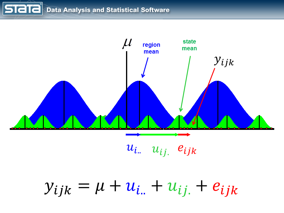
The equation for the variance-components model I fit had the form
\[y_{ijk} = mu + u_i.. + u_{ij.} + e_{ijk}\]
This model had three residuals, whereas the one-level model we just fit above had only one.
This time, let’s start with a two-level model. Let’s simulate a two-level dataset, a model for children nested within classrooms. We’ll index classrooms by i and children by j. The model is
\[y_{ij} = mu + u_{i.} + e_{ij}\]
For this toy model, let’s assume two classrooms with two students per classroom, meaning that we want to create a four-observation dataset, where the observations are students.
To create this four-observation dataset, we start by creating a two-observation dataset, where the observations are classrooms. Because there are two classrooms, we type
. clear
. set obs 2
. generate classroom = _n
From now on, we’ll refer to classroom as i. It’s easier to remember what variables mean if they have meaningful names.
Next, we’ll create a variable that contains each classroom’s random effect \(u_i\), which we’ll assume follows an N(0,3) distribution.
. generate u_i = rnormal(0,3)

. list

     +----------------------+
     | classr~m         u_i |
     |----------------------|
  1. |        1    .7491351 |
  2. |        2   -.0031386 |
     +----------------------+
We can now expand our data to include two children per classroom by typing
. expand 2

. list

     +----------------------+
     | classr~m         u_i |
     |----------------------|
  1. |        1    .7491351 |
  2. |        2   -.0031386 |
  3. |        1    .7491351 |
  4. |        2   -.0031386 |
     +----------------------+
Now, we can think of our observations as being students. We can create a child ID (we’ll call it child rather than j), and we can create each child’s residual \(e_{ij}\), which we will assume has an N(0,5) distribution:
. bysort classroom: generate child = _n

. generate e_ij = rnormal(0,5)

. list

     +------------------------------------------+
     | classr~m         u_i   child        e_ij |
     |------------------------------------------|
  1. |        1    .7491351       1    2.832674 |
  2. |        1    .7491351       2    1.487452 |
  3. |        2   -.0031386       1    6.598946 |
  4. |        2   -.0031386       2   -.3605778 |
     +------------------------------------------+
We now have nearly all the ingredients to calculate \(y_{ij}\):
\(y_{ij} = mu + u_{i.} + e_{ij}\)
We’ll assume mu is 70. We type
. generate y = 70 + u_i + e_ij

. list y classroom u_i child e_ij, sepby(classroom)

     +-----------------------------------------------------+
     |        y   classr~m         u_i   child        e_ij |
     |-----------------------------------------------------|
  1. | 73.58181          1    .7491351       1    2.832674 |
  2. | 72.23659          1    .7491351       2    1.487452 |
     |-----------------------------------------------------|
  3. | 76.59581          2   -.0031386       1    6.598946 |
  4. | 69.63628          2   -.0031386       2   -.3605778 |
     +-----------------------------------------------------+
Note that the random effect u_i is the same within each school, and each child has a different value for e_ij.
Our strategy was simple:
- Start with the top level of the data hierarchy.
- Create variables for the level ID and its random effect.
- Expand the data by the number of observations within that level.
- Repeat steps 2 and 3 until the bottom level is reached.
Let’s try this recipe for three-level data where children are nested within classrooms which are nested within schools. This time, I will index schools with i, classrooms with j, and children with k so that my model is
\[y_{ijk} = mu + u_{i..} + u_{ij.} + e_{ijk}\]
where
\(u_{i..}\) ~ N(0,2)
\(u_{ij.}\) ~ N(0,3)
\(u_{ijk}\) ~ N(0,5)
Let’s create data for
(level 3, i) 2 schools
(level 2, j) 2 classrooms in each school
(level 1, k) 2 students in most classrooms; 3 students in i==2 & j==2
Begin by creating the level-three data for the two schools:
. clear
. set obs 2
. generate school = _n
. generate u_i = rnormal(0,2)
. list school u_i

     +--------------------+
     | school         u_i |
     |--------------------|
  1. |      1    3.677312 |
  2. |      2   -3.193004 |
     +--------------------+
Next, we expand the data so that we have the two classrooms nested within each of the schools, and we create its random effect:
. expand 2
. bysort school: generate classroom = _n
. generate u_ij = rnormal(0,3)
. list school u_i classroom u_ij, sepby(school)

     +-------------------------------------------+
     | school         u_i   classr~m        u_ij |
     |-------------------------------------------|
  1. |      1    3.677312          1    .9811059 |
  2. |      1    3.677312          2   -3.482453 |
     |-------------------------------------------|
  3. |      2   -3.193004          1   -4.107915 |
  4. |      2   -3.193004          2   -2.450383 |
     +-------------------------------------------+
Finally, we expand the data so that we have three students in school 2’s classroom 2, and two students in all the other classrooms. Sorry for that complication, but I wanted to show you how to create unbalanced data.
In the previous examples, we’ve been typing things like expand 2, meaning double the observations. In this case, we need to do something different for school 2, classroom 2, namely,
. expand 3 if school==2 & classroom==2
and then we can just expand the rest:
. expand 2 if !(school==2 & clasroom==2)
Obviously, in a real simulation, you would probably want 16 to 25 students in each classroom. You could do something like that by typing
. expand 16+int((25-16+1)*runiform())
In any case, we will type
. expand 3 if school==2 & classroom==2

. expand 2 if !(school==2 & classroom==2)

. bysort school classroom: generate child = _n

. generate e_ijk = rnormal(0,5)

. generate y = 70 + u_i + u_ij + e_ijk

. list y school u_i classroom u_ij child e_ijk, sepby(classroom)

     +------------------------------------------------------------------------+
     |        y   school       u_i   classr~m        u_ij   child       e_ijk |
     |------------------------------------------------------------------------|
  1. | 76.72794        1  3.677312          1    .9811059       1    2.069526 |
  2. | 69.81315        1  3.677312          1    .9811059       2   -4.845268 |
     |------------------------------------------------------------------------|
  3. | 74.09565        1  3.677312          2   -3.482453       1    3.900788 |
  4. | 71.50263        1  3.677312          2   -3.482453       2    1.307775 |
     |------------------------------------------------------------------------|
  5. | 64.86206        2 -3.193004          1   -4.107915       1    2.162977 |
  6. | 61.80236        2 -3.193004          1   -4.107915       2   -.8967164 |
     |------------------------------------------------------------------------|
  7. | 66.65285        2 -3.193004          2   -2.450383       1    2.296242 |
  8. | 49.96139        2 -3.193004          2   -2.450383       2   -14.39522 |
  9. | 64.41605        2 -3.193004          2   -2.450383       3    .0594433 |
     +------------------------------------------------------------------------+
Regardless of how we generate the data, we must ensure that the school-level random effects u_i are the same within school and the classroom-level random effects u_ij are the same within classroom.
Concerning data construction, the example above we concocted to produce a dataset that would be easy to list. Let’s now create a dataset that is more reasonable:
\[y_{ijk} = mu + u_{i..} + u_{ij.} + e_{ijk}\]
where
\(u_{i..}\) ~ N(0,2)
\(u_{ij.}\) ~ N(0,3)
\(u_{ijk}\) ~ N(0,5)
Let’s create data for
(level 3, i) 6 schools
(level 2, j) 10 classrooms in each school
(level 1, k) 16-25 students
. clear
. set obs 6
. generate school = _n
. generate u_i = rnormal(0,2)
. expand 10
. bysort school: generate classroom = _n
. generate u_ij = rnormal(0,3)
. expand 16+int((25-16+1)*runiform())
. bysort school classroom: generate child = _n
. generate e_ijk = rnormal(0,5)
. generate y = 70 + u_i + u_ij + e_ijk
We can use the mixed command to fit the model with our simulated data.
. mixed y || school: || classroom: , stddev

Mixed-effects ML regression                     Number of obs      =      1217

-----------------------------------------------------------
                |   No. of       Observations per Group
 Group Variable |   Groups    Minimum    Average    Maximum
----------------+------------------------------------------
         school |        6        197      202.8        213
      classroom |       60         16       20.3         25
-----------------------------------------------------------

                                                Wald chi2(0)       =         .
Log likelihood = -3710.0673                     Prob > chi2        =         .

------------------------------------------------------------------------------
           y |      Coef.   Std. Err.      z    P>|z|     [95% Conf. Interval]
-------------+----------------------------------------------------------------
       _cons |   70.25941   .9144719    76.83   0.000     68.46707    72.05174
------------------------------------------------------------------------------

------------------------------------------------------------------------------
  Random-effects Parameters  |   Estimate   Std. Err.     [95% Conf. Interval]
-----------------------------+------------------------------------------------
school: Identity             |
                   sd(_cons) |   2.027064   .7159027      1.014487    4.050309
-----------------------------+------------------------------------------------
classroom: Identity          |
                   sd(_cons) |   2.814152   .3107647       2.26647    3.494178
-----------------------------+------------------------------------------------
                sd(Residual) |   4.828923   .1003814      4.636133     5.02973
------------------------------------------------------------------------------
LR test vs. linear regression:       chi2(2) =   379.37   Prob > chi2 = 0.0000
The parameter estimates from our simulated data match the parameters used to create the data pretty well: the estimate for _cons is 70.3, which is near 70; the estimated standard deviation for the school-level random effects is 2.02, which is near 2; the estimated standard deviation for the classroom-level random effects is 2.8, which is near 3; and the estimated standard deviation for the individual-level residuals is 4.8, which is near 5.
We’ve just done one reasonable simulation.
If we wanted to do a full simulation, we would need to do the above 100, 1,000, 10,000, or more times. We would put our code in a loop. And in that loop, we would keep track of whatever parameter interested us.
How to simulate three-level data with covariates
Usually, we’re more interested in estimating the effects of the covariates than in estimating the variance of the random effects. Covariates are typically binary (such as male/female), categorical (such as race), ordinal (such as education level), or continuous (such as age).
Let’s add some covariates to our simulated data. Our model is
\[y_{ijk} = mu + u_{i..} + u_{ij.} + e_{ijk}\]
where
\(u_{i..}\) ~ N(0,2)
\(u_{ij.}\) ~ N(0,3)
\(u_{ijk}\) ~ N(0,5)
We create data for
(level 3, i) 6 schools
(level 2, j) 10 classrooms in each school
(level 1, k) 16-25 students
Let’s add to this model
(level 3, school i) whether the school is in an urban environment
(level 2, classroom j) teacher’s experience (years)
(level 1, student k) student’s mother’s education level
We can create a binary covariate called urban at the school level that equals 1 if the school is located in an urban area and equals 0 otherwise.
. clear
. set obs 6
. generate school = _n
. generate u_i = rnormal(0,2)
. generate urban = runiform()<0.50
Here we assigned schools to one of the two groups with equal probability (runiform()<0.50), but we could have assigned 70% of the schools to be urban by typing
. generate urban = runiform()<0.70
At the classroom level, we could add a continuous covariate for the teacher's years of experience. We could generate this variable by using any of Stata's random-number functions (see help random_number_functions. In the example below, I've generated teacher's years of experience with a uniform distribution ranging from 5-20 years.
. expand 10
. bysort school: generate classroom = _n
. generate u_ij = rnormal(0,3)
. bysort school: generate teach_exp = 5+int((20-5+1)*runiform())
When we summarize our data, we see that teaching experience ranges from 6-20 years with an average of 13 years.
. summarize teach_exp

    Variable |       Obs        Mean    Std. Dev.       Min        Max
-------------+--------------------------------------------------------
   teach_exp |        60    13.21667    4.075939          6         20
At the child level, we could add a categorical/ordinal covariate for mother's highest level of education completed. After we expand the data and create the child ID and error variables, we can generate a uniformly distributed random variable, temprand, on the interval [0,1].
. expand 16+int((25-16+1)*runiform())
. bysort school classroom: generate child = _n
. generate e_ijk = rnormal(0,5)
. generate temprand = runiform()
We can assign children to different groups by using the egen command with cutpoints. In the example below, children whose value of temprand is in the interval [0,0.5) will be assigned to mother_educ==0, children whose value of temprand is in the interval [0.5,0.9) will be assigned to mother_educ==1, and children whose value of temprand is in the interval [0.9,1) will be assigned to mother_educ==2.
. egen mother_educ = cut(temprand), at(0,0.5, 0.9, 1) icodes
. label define mother_educ 0 "HighSchool" 1 "College" 2 ">College"
. label values mother_educ mother_educ
The resulting frequencies of each category are very close to the frequencies we specified in our egen command.
. tabulate mother_educ, generate(meduc)

mother_educ |      Freq.     Percent        Cum.
------------+-----------------------------------
 HighSchool |        602       50.17       50.17
    College |        476       39.67       89.83
   >College |        122       10.17      100.00
------------+-----------------------------------
      Total |      1,200      100.00
We used the option generate(meduc) in the tabulate command above to create indicator variables for each category of mother_educ. This will allow us to specify an effect size for each category when we create our outcome variable.
. summarize meduc*

    Variable |       Obs        Mean    Std. Dev.       Min        Max
-------------+--------------------------------------------------------
      meduc1 |      1200    .5016667    .5002057          0          1
      meduc2 |      1200    .3966667    .4894097          0          1
      meduc3 |      1200    .1016667    .3023355          0          1
Now, we can create an outcome variable called score by adding all our fixed and random effects together. We can specify an effect size (regression coefficient) for each fixed effect in our model.
. generate score = 70
        + (-2)*urban
        + 1.5*teach_exp
        + 0*meduc1
        + 2*meduc2
        + 5*meduc3
        + u_i + u_ij + e_ijk
I have specified that the grand mean is 70, urban schools will have scores 2 points lower than nonurban schools, and each year of teacher's experience will add 1.5 points to the students score.
Mothers whose highest level of education was high school (meduc1==1) will serve as the referent category for mother_educ(mother_educ==0). The scores of children whose mother completed college (meduc2==1 and mother_educ==1) will be 2 points higher than the children in the referent group. And the scores of children whose mother completed more than college (meduc3==1 and mother_educ==2) will be 5 points higher than the children in the referent group. Now, we can use the mixed command to fit a model to our simulated data. We used the indicator variables meduc1-meduc3 to create the data, but we will use the factor variable i.mother_educ to fit the model.
. mixed score urban teach_exp i.mother_educ  || school: ||
                                             classroom: , stddev baselevel

Mixed-effects ML regression                     Number of obs      =      1259

-----------------------------------------------------------
                |   No. of       Observations per Group
 Group Variable |   Groups    Minimum    Average    Maximum
----------------+------------------------------------------
         school |        6        200      209.8        217
      classroom |       60         16       21.0         25
-----------------------------------------------------------

                                                Wald chi2(4)       =    387.64
Log likelihood = -3870.5395                     Prob > chi2        =    0.0000

------------------------------------------------------------------------------
       score |      Coef.   Std. Err.      z    P>|z|     [95% Conf. Interval]
-------------+----------------------------------------------------------------
       urban |  -2.606451    2.07896    -1.25   0.210    -6.681138    1.468237
   teach_exp |   1.584759    .096492    16.42   0.000     1.395638     1.77388
             |
 mother_educ |
 HighSchool  |          0  (base)
    College  |   2.215281   .3007208     7.37   0.000     1.625879    2.804683
   >College  |   5.065907   .5237817     9.67   0.000     4.039314      6.0925
             |
       _cons |   68.95018   2.060273    33.47   0.000     64.91212    72.98824
------------------------------------------------------------------------------

------------------------------------------------------------------------------
  Random-effects Parameters  |   Estimate   Std. Err.     [95% Conf. Interval]
-----------------------------+------------------------------------------------
school: Identity             |
                   sd(_cons) |   2.168154   .7713944      1.079559    4.354457
-----------------------------+------------------------------------------------
classroom: Identity          |
                   sd(_cons) |    3.06871   .3320171      2.482336    3.793596
-----------------------------+------------------------------------------------
                sd(Residual) |   4.947779   .1010263      4.753681    5.149802
------------------------------------------------------------------------------
LR test vs. linear regression:       chi2(2) =   441.25   Prob > chi2 = 0.0000
"Close" is in the eye of the beholder, but to my eyes, the parameter estimates look remarkably close to the parameters that were used to simulate the data. The parameter estimates for the fixed part of the model are -2.6 for urban (parameter = -2), 1.6 for teach_exp (parameter = 1.5), 2.2 for the College category of mother_educ (parameter = 2), 5.1 for the >College category of mother_educ (parameter = 5), and 69.0 for the intercept (parameter = 70). The estimated standard deviations for the random effects are also very close to the simulation parameters. The estimated standard deviation is 2.2 (parameter = 2) at the school level, 3.1 (parameter = 3) at the classroom level, and 4.9 (parameter = 5) at the child level.
Some of you may disagree that the parameter estimates are close. My reply is that it doesn't matter unless you're simulating a single dataset for demonstration purposes. If you are, simply simulate more datasets until you get one that looks close enough for you. If you are simulating data to check coverage probabilities or to estimate statistical power, you will be averaging over thousands of simulated datasets and the results of any one of those datasets won't matter.
How to simulate longitudinal data with random slopes
Longitudinal data are often conceptualized as multilevel data where the repeated observations are nested within individuals. The main difference between ordinary multilevel models and multilevel models for longitudinal data is the inclusion of a random slope. If you are not familiar with random slopes, you can learn more about them in a blog entry I wrote last year (Multilevel linear models in Stata, part 2: Longitudinal data).
Simulating longitudinal data with a random slope is much like simulating two-level data, with a couple of modifications. First, the bottom level will be observations within person. Second, there will be an interaction between time (age) and a person-level random effect. So we will generate data for the following model:
\[weight_{ij} = mu + age_{ij} + u_{0i.} + age*u_{1i.} + e_{ij}\]
where
\(u_{0i.}\) ~ N(0,3) \(u_{1i.}\) ~ N(0,1) \(e_{ij}\) ~ N(0,2)
Let's begin by simulating longitudinal data for 300 people.
. clear
. set obs 300
. gen person = _n
For longitudinal data, we must create two person-level random effects: the variable u_0i is analogous to the random effect we created earlier, and the variable u_1i is the random effect for the slope over time.
. generate u_0i = rnormal(0,3)
. generate u_1i = rnormal(0,1)
Let's expand the data so that there are five observations nested within each person. Rather than create an observation-level identification number, let's create a variable for age that ranges from 12 to 16 years,
. expand 5
. bysort person: generate age = _n + 11
and create an observation-level error term from an N(0,2) distribution:
. generate e_ij = rnormal(0,2)

. list person u_0i u_1i age e_ij if person==1

      +-------------------------------------------------+
      | person       u_0i        u_1i   age        e_ij |
      |-------------------------------------------------|
   1. |      1   .9338312   -.3097848    12    1.172153 |
   2. |      1   .9338312   -.3097848    13    2.935366 |
   3. |      1   .9338312   -.3097848    14   -2.306981 |
   4. |      1   .9338312   -.3097848    15   -2.148335 |
   5. |      1   .9338312   -.3097848    16   -.4276625 |
      +-------------------------------------------------+
The person-level random effects u_0i and u_1i are the same at all ages, and the observation-level random effects e_ij are different at each age. Now we're ready to generate an outcome variable called weight, measured in kilograms, based on the following model:
\[weight_{ij} = 3 + 3.6*age_{ij} + u_{0i} + age*u_{1i} + e_{ij}\]
. generate weight = 3 + 3.6*age + u_0i + age*u_1i + e_ij
The random effect u_1i is multiplied by age, which is why it is called a random slope. We could rewrite the model as
\[weight_{ij} = 3 + age_{ij}*(3.6 + u_{1i}) + u_{01} + e_{ij}\]
Note that for each year of age, a person's weight will increase by 3.6 kilograms plus some random amount specified by u_1j. In other words,the slope for age will be slightly different for each person.
We can use the mixed command to fit a model to our data:
. mixed weight age || person: age , stddev

Mixed-effects ML regression                     Number of obs      =      1500
Group variable: person                          Number of groups   =       300

                                                Obs per group: min =         5
                                                               avg =       5.0
                                                               max =         5


                                                Wald chi2(1)       =   3035.03
Log likelihood = -3966.3842                     Prob > chi2        =    0.0000

------------------------------------------------------------------------------
      weight |      Coef.   Std. Err.      z    P>|z|     [95% Conf. Interval]
-------------+----------------------------------------------------------------
         age |   3.708161   .0673096    55.09   0.000     3.576237    3.840085
       _cons |   2.147311   .5272368     4.07   0.000     1.113946    3.180676
------------------------------------------------------------------------------

------------------------------------------------------------------------------
  Random-effects Parameters  |   Estimate   Std. Err.     [95% Conf. Interval]
-----------------------------+------------------------------------------------
person: Independent          |
                     sd(age) |   .9979648   .0444139      .9146037    1.088924
                   sd(_cons) |    3.38705   .8425298      2.080103    5.515161
-----------------------------+------------------------------------------------
                sd(Residual) |   1.905885   .0422249      1.824897    1.990468
------------------------------------------------------------------------------
LR test vs. linear regression:       chi2(2) =  4366.32   Prob > chi2 = 0.0000
The estimate for the intercept _cons = 2.1 is not very close to the original parameter value of 3, but the estimate of 3.7 for age is very close (parameter = 3.6). The standard deviations of the random effects are also very close to the parameters used to simulate the data. The estimate for the person level _cons is 2.1 (parameter = 2), the person-level slope is 0.997 (parameter = 1), and the observation-level residual is 1.9 (parameter = 2).
How to simulate longitudinal data with structured errors
Longitudinal data often have an autoregressive pattern to their errors because of the sequential collection of the observations. Measurements taken closer together in time will be more similar than measurements taken further apart in time. There are many patterns that can be used to descibe the correlation among the errors, including autoregressive, moving average, banded, exponential, Toeplitz, and others (see help mixed##rspec).
Let's simulate a dataset where the errors have a Toeplitz structure, which I will define below.
We begin by creating a sample with 500 people with a person-level random effect having an N(0,2) distribution.
. clear
. set obs 500
. gen person = _n
. generate u_i = rnormal(0,2)
Next, we can use the drawnorm command to create error variables with a Toeplitz pattern.
A Toeplitz 1 correlation matrix has the following structure:
. matrix V = ( 1.0, 0.5, 0.0, 0.0, 0.0  \     ///
               0.5, 1.0, 0.5, 0.0, 0.0  \     ///
               0.0, 0.5, 1.0, 0.5, 0.0  \     ///
               0.0, 0.0, 0.5, 1.0, 0.5  \     ///
               0.0, 0.0, 0.0, 0.5, 1.0 )

. matrix list V

symmetric V[5,5]
    c1  c2  c3  c4  c5
r1   1
r2  .5   1
r3   0  .5   1
r4   0   0  .5   1
r5   0   0   0  .5   1
The correlation matrix has 1s on the main diagonal, and each pair of contiguous observations will have a correlation of 0.5. Observations more than 1 unit of time away from each other are assumed to be uncorrelated.
We must also define a matrix of means to use the drawnorm command.
. matrix M = (0 \ 0 \ 0 \ 0 \ 0)

. matrix list M

M[5,1]
    c1
r1   0
r2   0
r3   0
r4   0
r5   0
Now, we're ready to use the drawnorm command to create five error variables that have a Toeplitz 1 structure.
. drawnorm e1 e2 e3 e4 e5, means(M) cov(V)

. list in 1/2

     +---------------------------------------------------------------------------+
     | person        u_i         e1         e2        e3          e4          e5 |
     |---------------------------------------------------------------------------|
  1. |      1   5.303562  -1.288265  -1.201399   .353249    .0495944   -1.472762 |
  2. |      2  -.0133588   .6949759    2.82179  .7195075   -1.032395    .1995016 |
     +---------------------------------------------------------------------------+
Let's estimate the correlation matrix for our simulated data to verify that our simulation worked as we expected.
. correlate e1-e5
(obs=300)

             |       e1       e2       e3       e4       e5
-------------+---------------------------------------------
          e1 |   1.0000
          e2 |   0.5542   1.0000
          e3 |  -0.0149   0.4791   1.0000
          e4 |  -0.0508  -0.0364   0.5107   1.0000
          e5 |   0.0022  -0.0615   0.0248   0.4857   1.0000
The correlations are 1 along the main diagonal, near 0.5 for the contiguous observations, and near 0 otherwise.
Our data are currently in wide format, and we need them in long format to use the mixed command. We can use the reshape command to convert our data from wide to long format. If you are not familiar with the reshape command, you can learn more about it by typing help reshape.
. reshape long e, i(person) j(time)
(note: j = 1 2 3 4 5)

Data                               wide   ->   long
-----------------------------------------------------------------------------
Number of obs.                      300   ->    1500
Number of variables                   7   ->       4
j variable (5 values)                     ->   time
xij variables:
                           e1 e2 ... e5   ->   e
-----------------------------------------------------------------------------
Now, we are ready to create our age variable and the outcome variable weight.
. bysort person: generate age = _n + 11
. generate weight = 3 + 3.6*age + u_i + e

. list weight person u_i time age e if person==1

      +-------------------------------------------------------+
      |   weight   person        u_i   time   age           e |
      |-------------------------------------------------------|
   1. |  50.2153        1   5.303562      1    12   -1.288265 |
   2. | 53.90216        1   5.303562      2    13   -1.201399 |
   3. | 59.05681        1   5.303562      3    14     .353249 |
   4. | 62.35316        1   5.303562      4    15    .0495944 |
   5. |  64.4308        1   5.303562      5    16   -1.472762 |
      +-------------------------------------------------------+
We can use the mixed command to fit a model to our simulated data.
. mixed weight age || person:, residual(toeplitz 1, t(time)) , stddev

Mixed-effects ML regression                     Number of obs      =      1500
Group variable: person                          Number of groups   =       300

                                                Obs per group: min =         5
                                                               avg =       5.0
                                                               max =         5

                                                Wald chi2(1)       =  33797.58
Log likelihood = -2323.9389                     Prob > chi2        =    0.0000

------------------------------------------------------------------------------
      weight |      Coef.   Std. Err.      z    P>|z|     [95% Conf. Interval]
-------------+----------------------------------------------------------------
         age |   3.576738   .0194556   183.84   0.000     3.538606     3.61487
       _cons |   3.119974   .3244898     9.62   0.000     2.483985    3.755962
------------------------------------------------------------------------------

------------------------------------------------------------------------------
  Random-effects Parameters  |   Estimate   Std. Err.     [95% Conf. Interval]
-----------------------------+------------------------------------------------
person: Identity             |
                   sd(_cons) |   3.004718   .1268162      2.766166    3.263843
-----------------------------+------------------------------------------------
Residual: Toeplitz(1)        |
                        rho1 |   .4977523   .0078807      .4821492    .5130398
                       sd(e) |   .9531284   .0230028      .9090933    .9992964
------------------------------------------------------------------------------
LR test vs. linear regression:       chi2(2) =  3063.87   Prob > chi2 = 0.0000
Again, our parameter estimates match the parameters that were used to simulate the data very closely.
The parameter estimate is 3.6 for age (parameter = 3.6) and 3.1 for _cons (parameter = 3). The estimated standard deviations of the person-level random effect is 3.0 (parameter = 3). The estimated standard deviation for the errors is 0.95 (parameter = 1), and the estimated correlation for the Toeplitz structure is 0.5 (parameter = 0.5).
Conclusion
I hope I've convinced you that simulating multilevel/longitudinal data is easy and useful. The next time you find yourself teaching a class or giving a talk that requires multilevel examples, try simulating the data. And if you need to calculate statistical power for a multilevel or longitudinal model, consider simulations.