Cointegration or spurious regression?
\(\newcommand{\betab}{\boldsymbol{\beta}}\)Time-series data often appear nonstationary and also tend to comove. A set of nonstationary series that are cointegrated implies existence of a long-run equilibrium relation. If such an equlibrium does not exist, then the apparent comovement is spurious and no meaningful interpretation ensues.
Analyzing multiple nonstationary time series that are cointegrated provides useful insights about their long-run behavior. Consider long- and short-term interest rates such as the yield on a 30-year and a 3-month U.S. Treasury bond. According to the expectations hypothesis, long-term interest rates are determined by the average of expected future short-term rates. This implies that the yields on the two bonds cannot deviate from one another over time. Thus, if the two yields are cointegrated, any influence to the short-term rate leads to adjustments in the long-term interest rate. This has important implications in making various policy or investment decisions.
In a cointegration analysis, we begin by regressing a nonstationary variable on a set of other nonstationary variables. Suprisingly, in finite samples, regressing a nonstationary series with another arbitrary nonstationary series usually results in significant coefficients with a high \(R^2\). This gives a false impression that the series may be cointegrated, a phenomenon commonly known as spurious regression.
In this post, I use simulated data to show the asymptotic properties of an ordinary least-squares (OLS) estimator under cointegration and spurious regression. I then perform a test for cointegration using the Engle and Granger (1987) method. These exercises provide a good first step toward understanding cointegrated processes.
Cointegration
For ease of exposition, I consider two variables, \(y_t\) and \(x_t\), that are integrated of order 1 or I(1). They can be transformed to a stationary or I(0) series by taking first differences.
The variables \(y_t\) and \(x_t\) are cointegrated if their linear combination is I(0). This implies \(\betab [y_t,x_t]’ = e_t\), where \(\betab\) is the cointegrating vector and \(e_t\) is a stationary equilibrium error. Typically, with the addition of more variables, more than one cointegrating vector may exist. Nonetheless, the Engle–Granger method assumes a single cointegrating vector regardless of the number of variables being modeled.
A normalizing assumption such as \(\betab = (1,-\beta)\) is made to uniquely identify the cointegrating vector using OLS. This type of normalization specifies which variables occur on the left- and right-hand side of the equation. In the case of cointegrated variables, the choice of normalization is irrelevant asymptotically. Nonetheless, in practice, they are typically guided by some theory that dictates their relationship. The normalization in the current application leads to the following regression specification.
\begin{equation}
\label{eq1}
y_t = \beta x_t + e_t
\tag{1}
\end{equation}
The equation above describes the long-run relation between \(y_t\) and \(x_t\). This is also referred to as a “static” regression because no other dynamics in the variables and serial correlation in the error term are assumed.
The OLS estimator is given by \(\hat{\beta}= \frac{\sum_{t=1}^T y_t x_t}{\sum_{t=1}^T x^2_t}\). Because \(y_t\) and \(x_t\) are both I(1) processes, the numerator and denominator converge to complicated functions of Brownian motions as \(T\to \infty\). However, \(\hat{\beta}\) still consistently estimates the true \(\beta\) regardless of whether \(x_t\) is correlated with \(e_t\). In fact, the estimator is superconsistent, which implies it converges to the true value at a faster rate than an OLS estimator of a regression on stationary series. Inference on \(\hat{\beta}\) is not straightforwad because its asymptotic distribution is nonstandard and also depends on whether deterministic terms such as constant and time trend are specified.
Monte Carlo simulations
I perform Monte Carlo simulations (MCS) with 1,000 replications to plot the empirical densities of the OLS estimator \(\hat{\beta}\) under spurious regression and cointegration. In the case of spurious regression, the empirical density of \(\hat{\beta}\) does not shrink toward the true value even after increasing the sample size. This implies that the OLS estimator is inconsistent. On the other hand, if the series are cointegrated, we expect the empirical density of \(\hat{\beta}\) to converge to its true value.
Data-generating process for spurious regression
I generate \(y_t\) and \(x_t\) according to the following specification,
\begin{align}
\label{eq2}
y_t &= 0.7 x_t + e_t \\
\nonumber
x_t &= x_{t-1} + \nu_{xt}\\
\nonumber
e_t &= e_{t-1} + \nu_{yt} \tag{2}
\end{align}
where \(\nu_{xt}\) and \(\nu_{yt}\) are IID N(0,1). \(x_t\) and \(e_t\) are independent random walks. This is a spurious regression because the linear combination \(y_t – 0.7x_t = e_t\) is an I(1) process.
Data-generating process for cointegration
I generate \(y_t\) and \(x_t\) according to the following specification,
\begin{align}
\label{eq3}
y_t &= 0.7 x_t + e_{yt} \\
\nonumber
x_t &= x_{t-1} + e_{xt} \tag{3}
\end{align}
where \(x_t\) is the only I(1) process. I allow for contemporaneous correlation as well as serial correlation by generating the error terms \(e_{yt}\) and \(e_{xt}\) as a vector moving average (VMA) process with 1 lag. The VMA model is given by
\begin{align*}
e_{yt} &= 0.3 \nu_{yt-1} + 0.4 \nu_{xt-1} + \nu_{yt} \\
e_{xt} &= 0.7 \nu_{yt-1} + 0.1 \nu_{xt-1} + \nu_{xt} \\
\end{align*}
where \(\nu_{yt}\) and \(\nu_{xt}\) are drawn from a normal distribution with mean 0 and variance matrix \({\bf \Sigma} = \left[\begin{matrix} 1 & 0.7 \\ 0.7 & 1.5 \end{matrix}\right]\). The graph below plots the empirical densities. The code for performing the simulations is provided in the Appendix.
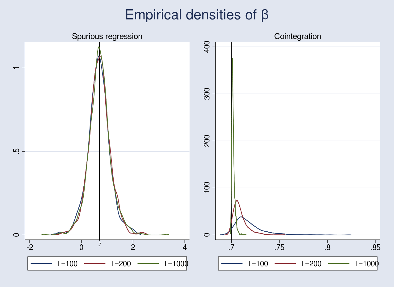
In the case of spurious regression, the OLS estimator is inconsistent because it does not converge to its true value even after increasing the sample size from 100 to 1,000. The vertical line at 0.7 represents the true value of \(\beta\). Moreover, in finite samples, the coefficients in a spurious regression are usually significant with a high \(R^2\). In fact, Phillips (1986) showed that the \(t\) and \(F\) statistics diverge in distribution as \(T\to \infty\), thus making any inferences invalid.
In the case of cointegration, I artificially introduced serial correlation in the error terms in the data-generating process. This led to a biased estimate as seen in the graph above for a sample size of 100, which improves slightly as the sample size increases to 200. Remarkably, the OLS estimator converges to its true value as we increase the sample size to 1,000. While consistency is an important property, we still cannot perform inference on \(\hat{\beta}\) because of its nonstandard asymptotic distribution.
Testing for cointegration
We saw in the previous section that the OLS estimator is consistent if the series are cointegrated. This is true even when we fail to account for serial correlation in the error terms. To test for cointegration, we can construct residuals based on the static regression and test for the presence of unit root. If the series are cointegrated, the estimated residuals will be close to being stationary. This is the approach in the Engle–Granger two-step method. The first step estimates \(\beta\) in \eqref{eq1} by OLS followed by testing for unit root in the residuals. Tests such as the augmented Dickey–Fuller (ADF) or Phillips–Perron (PP) can be performed on the residuals. Refer to an earlier post for a discussion of these tests.
The null and alternative hypotheses for testing cointegration are as follows:
\[
H_o: e_t = I(1) \qquad H_a: e_t = I(0)
\]
The null hypothesis states that \(e_t\) is nonstationary, which implies no cointegration between \(y_t\) and \(x_t\). The alternative hypothesis states that \(e_t\) is stationary and implies cointegration.
If the true cointegrating vector \(\betab\) is known, then we simply plug its value in (1) and obtain the \(e_t\) series. We then apply the ADF test to \(e_t\). The test statistic will have the standard DF distribution.
In the case of an unknown cointegrating vector \(\betab\), the ADF test statistic based on the estimated residuals does not follow the standard DF distribution under the null hypothesis of no cointegration (Phillips and Ouliaris 1990). Furthermore, Hansen (1992) shows that the distribution of the ADF statistic also depends on whether \(y_t\) and \(x_t\) contain deterministic terms such as constants and time trends. Hamilton (1994, 766) provides critical values for making inference in such cases.
Example
I have two datasets that I saved while performing MCS in the previous section. spurious.dta consists of two variables, \(y_t\) and \(x_t\), generated according to the spurious regression equations in (2). coint.dta also consists of \(y_t\) and \(x_t\), generated using the cointegration equation in (3).
First, I test for cointegration in spurious.dta.
. use spurious, clear

. reg y x, nocons

      Source |       SS           df       MS      Number of obs   =       100
-------------+----------------------------------   F(1, 99)        =      6.20
       Model |  63.4507871         1  63.4507871   Prob > F        =    0.0144
    Residual |  1013.32308        99  10.2355867   R-squared       =    0.0589
-------------+----------------------------------   Adj R-squared   =    0.0494
       Total |  1076.77387       100  10.7677387   Root MSE        =    3.1993

------------------------------------------------------------------------------
           y |      Coef.   Std. Err.      t    P>|t|     [95% Conf. Interval]
-------------+----------------------------------------------------------------
           x |  -.1257176   .0504933    -2.49   0.014    -.2259073   -.0255279
------------------------------------------------------------------------------
The coefficient on x is negative and significant. I use predict with the resid option to generate the residuals and perform an ADF test using the dfuller command. I use the noconstant option to supress the constant term in the regression and lags(2) to adjust for serial correlation. The noconstant option in the dfuller command implies fitting a random walk model.
. predict spurious_resd, resid

. dfuller spurious_resd, nocons lags(2)

Augmented Dickey-Fuller test for unit root         Number of obs   =        97

                               ---------- Interpolated Dickey-Fuller ---------
                  Test         1% Critical       5% Critical      10% Critical
               Statistic           Value             Value             Value
------------------------------------------------------------------------------
 Z(t)             -1.599            -2.601            -1.950            -1.610
As mentioned earlier, the critical values of the DF distribution may not be used in this case. The 5% critical value provided in the first row of Hamilton (1994, 766) under case 1 in table B.9 is \(-\)2.76. The test statistic of \(-\)1.60 in this case implies failure to reject the null hypothesis of no cointegration.
I perform the same two-step method for coint.dta below.
. use coint, clear

. reg y x, nocons

      Source |       SS           df       MS      Number of obs   =       100
-------------+----------------------------------   F(1, 99)        =   3148.28
       Model |  4411.48377         1  4411.48377   Prob > F        =    0.0000
    Residual |   138.72255        99  1.40123788   R-squared       =    0.9695
-------------+----------------------------------   Adj R-squared   =    0.9692
       Total |  4550.20632       100  45.5020632   Root MSE        =    1.1837

------------------------------------------------------------------------------
           y |      Coef.   Std. Err.      t    P>|t|     [95% Conf. Interval]
-------------+----------------------------------------------------------------
           x |   .7335899   .0130743    56.11   0.000     .7076477    .7595321
------------------------------------------------------------------------------

. predict coint_resd, resid

. dfuller coint_resd, nocons lags(2)

Augmented Dickey-Fuller test for unit root         Number of obs   =        97

                               ---------- Interpolated Dickey-Fuller ---------
                  Test         1% Critical       5% Critical      10% Critical
               Statistic           Value             Value             Value
------------------------------------------------------------------------------
 Z(t)             -5.955            -2.601            -1.950            -1.610
Comparing the DF test statistic of \(-\)5.95 with the appropriate critical value of \(-\)2.76, I reject the null hypothesis of no cointegration at the 5% level.
Conclusion
In this post, I performed MCS to show the consistency of the OLS estimator under cointegration. I used the Engle–Granger two-step approach to test for cointegration in simulated data.
References
Engle, R. F., and C. W. J. Granger. 1987. Co-integration and error correction: Representation, estimation, and testing. Econometrica 55: 251–276.
Hamilton, J. D. 1994. Time Series Analysis. Princeton: Princeton University Press.
Hansen, B. E. 1992. Effcient estimation and testing of cointegrating vectors in the presence of deterministic trends. Journal of Econometrics 53: 87–121.
Phillips, P. C. B. 1986. Understanding spurious regressions in econometrics. Journal of Econometrics 33: 311–340.
Phillips, P. C. B., and S. Ouliaris. 1990. Asymptotic properties of residual based tests for cointegration. Econometrica 58: 165–193.
Appendix
Code for spurious regression
The following code performs an MCS for a sample size of 100.
cscript
set seed 2016

local MC = 1000

quietly postfile spurious beta_t100 using t100, replace

forvalues i=1/`MC' {
        quietly {
                drop _all

                set obs 100
                gen time = _n
                tsset time

                gen nu_y = rnormal(0,0.7)
                gen nu_x = rnormal(0,1.5)

                gen err_y = nu_y in 1
                gen err_x = nu_x in 1
                replace err_y = l.err_y + nu_y in 2/l
                replace err_x = l.err_x + nu_x in 2/l

                gen y = err_y in 1
                gen x = err_x
                replace y = 0.7*x + err_y in 2/l
                if (`i'==1) save spurious, replace
                qui reg y x, nocons
        }
                post spurious (_b[x])
}
postclose spurious
Code for cointegration
The following code performs an MCS for a sample size of 100.
cscript
set seed 2016

local MC = 1000

quietly postfile coint beta_t100 using t100, replace

forvalues i=1/`MC' {
        quietly {
                drop _all

                set obs 100
                gen time = _n
                tsset time

                matrix V = (1,0.7\0.7,1.5)
                drawnorm nu_y nu_x, cov(V)

                gen err_y = nu_y in 1
                gen err_x = nu_x in 1
                replace err_y = 0.3*l.nu_y + 0.4*l.nu_x ///
                        + nu_y in 2/l
                replace err_x = 0.7*l.nu_y + 0.1*l.nu_x ///
                        + nu_x in 2/l

                gen x = err_x in 1
                replace x = l.x + err_x in 2/l
                gen y = 0.7*x + err_y
                if (`i'==1) save coint, replace
                qui reg y x, nocons
        }
                post coint (_b[x])
}
postclose coint
Combining graphs
Assuming you have run an MCS for sample sizes of 200 and 1,000, you may combine the graph using the following code block.
/*Spurious regression*/
use t100, clear
quietly merge 1:1 _n using t200
drop _merge
quietly merge 1:1 _n using t1000
drop _merge
kdensity beta_t100, n(1000) generate(x_100 f_100) ///
        kernel(gaussian) nograph
label variable f_100 "T=100"
kdensity beta_t200, n(1000) generate(x_200 f_200) ///
        kernel(gaussian) nograph
label variable f_200 "T=200"
kdensity beta_t1000, n(1000) generate(x_1000 f_1000) ///
        kernel(gaussian) nograph
label variable f_1000 "T=1000"
graph twoway (line f_100 x_100) (line f_200 x_200) ///
        (line f_1000 x_1000), legend(rows(1))      ///
        subtitle("Spurious regression")            ///
        saving(spurious, replace) xmlabel(0.7)     ///
        xline(0.7, lcolor(black)) nodraw

/*Cointegration*/
use t100, clear
quietly merge 1:1 _n using t200
drop _merge
quietly merge 1:1 _n using t1000
drop _merge
kdensity beta_t100, n(1000) generate(x_100 f_100) ///
        kernel(gaussian) nograph
label variable f_100 "T=100"
kdensity beta_t200, n(1000) generate(x_200 f_200) ///
        kernel(gaussian) nograph
label variable f_200 "T=200"
kdensity beta_t1000, n(1000) generate(x_1000 f_1000) ///
        kernel(gaussian) nograph
label variable f_1000 "T=1000"
graph twoway (line f_100 x_100) (line f_200 x_200) ///
        (line f_1000 x_1000), legend(rows(1))      ///
        subtitle("Cointegration")                  ///
        saving(cointegration, replace)             ///
        xline(0.7, lcolor(black)) nodraw

graph combine spurious.gph cointegration.gph,      ///
      title("Empirical densities of {&beta}")