Programming an estimation command in Stata: A review of nonlinear optimization using Mata
\(\newcommand{\betab}{\boldsymbol{\beta}}
\newcommand{\xb}{{\bf x}}
\newcommand{\yb}{{\bf y}}
\newcommand{\gb}{{\bf g}}
\newcommand{\Hb}{{\bf H}}
\newcommand{\thetab}{\boldsymbol{\theta}}
\newcommand{\Xb}{{\bf X}}
\)I review the theory behind nonlinear optimization and get more practice in Mata programming by implementing an optimizer in Mata. In real problems, I recommend using the optimize() function or moptimize() function instead of the one I describe here. In subsequent posts, I will discuss optimize() and moptimize(). This post will help you develop your Mata programming skills and will improve your understanding of how optimize() and moptimize() work.
This is the seventeenth post in the series Programming an estimation command in Stata. I recommend that you start at the beginning. See Programming an estimation command in Stata: A map to posted entries for a map to all the posts in this series.
A quick review of nonlinear optimization
We want to maximize a real-valued function \(Q(\thetab)\), where \(\thetab\) is a \(p\times 1\) vector of parameters. Minimization is done by maximizing \(-Q(\thetab)\). We require that \(Q(\thetab)\) is twice, continuously differentiable, so that we can use a second-order Taylor series to approximate \(Q(\thetab)\) in a neighborhood of the point \(\thetab_s\),
\[
Q(\thetab) \approx Q(\thetab_s) + \gb_s'(\thetab -\thetab_s)
+ \frac{1}{2} (\thetab -\thetab_s)’\Hb_s (\thetab -\thetab_s)
\tag{1}
\]
where \(\gb_s\) is the \(p\times 1\) vector of first derivatives of \(Q(\thetab)\) evaluated at \(\thetab_s\) and \(\Hb_s\) is the \(p\times p\) matrix of second derivatives of \(Q(\thetab)\) evaluated at \(\thetab_s\), known as the Hessian matrix.
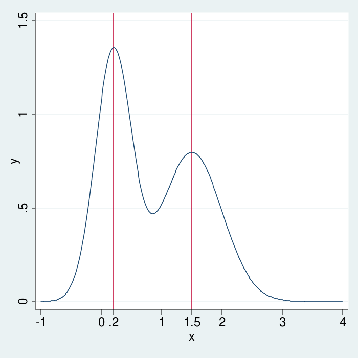
Nonlinear maximization algorithms start with a vector of initial values and produce a sequence of updated values that converge to the parameter vector that maximizes the objective function. The algorithms I discuss here can only find local maxima. The function in figure 1 has a local maximum at .2 and another at 1.5. The global maximum is at .2.
Figure 1: Local maxima
Each update is produced by finding the \(\thetab\) that maximizes the approximation on the right-hand side of equation (1) and letting it be \(\thetab_{s+1}\). To find the \(\thetab\) that maximizes the approximation, we set to \({\bf 0}\) the derivative of the right-hand side of equation (1) with respect to \(\thetab\),
\[
\gb_s + \Hb_s (\thetab -\thetab_s) = {\bf 0}
\tag{2}
\]
Replacing \(\thetab\) with \(\thetab_{s+1}\) and solving yields the update rule for \(\thetab_{s+1}\).
\[
\thetab_{s+1} = \thetab_s – \Hb_s^{-1} \gb_s
\tag{3}
\]
Note that the update is uniquely defined only if the Hessian matrix \(\Hb_s\) is full rank. To ensure that we have a local maximum, we will require that the Hessian be negative definite at the optimum, which also implies that the symmetric Hessian is full rank.
The update rule in equation (3) does not guarantee that \(Q(\thetab_{s+1})>Q(\thetab_s)\). We want to accept only those \(\thetab_{s+1}\) that do produce such an increase, so in practice, we use
\[
\thetab_{s+1} = \thetab_s – \lambda \Hb_s^{-1} \gb_s
\tag{4}
\]
where \(\lambda\) is the step size. In the algorithm presented here, we start with \(\lambda\) equal to \(1\) and, if necessary, decrease \(\lambda\) until we find a value that yields an increase.
The previous sentence is vague. I clarify it by writing an algorithm in Mata. Suppose that real scalar Q( real vector theta ) is a Mata function that returns the value of the objective function at a value of the parameter vector theta. For the moment, suppose that g_s is the vector of derivatives at the current theta, denoted by theta_s, and that Hi_s is the inverse of the Hessian matrix at theta_s. These definitions allow us to define the update function
real vector tupdate(                 ///
	real scalar lambda,          ///
	real vector theta_s,         ///
	real vector g_s,             ///
	real matrix Hi_s)
{
	return (theta_s - lambda*Hi_s*g_s)
}
For specified values of lambda, theta_s, g_s, and Hi_s, tupdate() returns a candidate value for theta_s1. But we only accept candidate values of theta_s1 that yield an increase, so instead of using tupdate() to get an update, we would use GetUpdate().
real vector GetUpdate(            ///
    real vector theta_s,          ///
    real vector g_s,              ///
    real matrix Hi_s)
{
    lambda = 1
    theta_s1 = tupdate(lambda, thetas, g_s, Hi_s)
    while ( Q(theta_s1) < Q(theta_s) ) {
        lambda   = lambda/2
        theta_s1 = tupdate(lambda, thetas, g_s, Hi_s)
    }
    return(theta_s1)
}
GetUpdate() starts by getting a candidate value for theta_s1 when lambda = 1. GetUpdate() returns this candidate theta_s1 if it produces an increase in Q(). Otherwise, GetUpdate() divides lambda by 2 and gets another candidate theta_s1 until it finds a candidate that produces an increase in Q(). GetUpdate() returns the first candidate that produces an increase in Q().
While these functions clarify the ambiguities in the original vague statement, GetUpdate() makes the unwise assumption that there is always a lambda for which the candidate theta_s1 produces an increase in Q(). The version of GetUpdate() in code block 3 does not make this assumption, it exits with an error if lambda is too small; less than \(10^{-11}\).
real vector GetUpdate(            ///
    real vector theta_s,          ///
    real vector g_s,              ///
    real matrix Hi_s)
{
    lambda = 1
    theta_s1 = tupdate(lambda, thetas, g_s, Hi_s)
    while ( Q(theta_s1) < Q(theta_s) ) {
        lambda   = lambda/2
        if (lambda < 1e-11) {
            printf("{red}Cannot find parameters that produce an increase.\n")
            exit(error(3360))
        }
        theta_s1 = tupdate(lambda, thetas, g_s, Hi_s)
    }
    return(theta_s1)
}
An outline of our algorithm for nonlinear optimization is the following:
- Select initial values for parameter vector.
- If current parameters set vector of derivatives of Q() to zero, go to (3); otherwise go to (A).
- Use GetUpdate() to get new parameter values.
- Calculate g_s and Hi_s at parameter values from (A).
- Go to (2).
- Display results.
Code block 4 contains a Mata version of this algorithm.
theta_s  =  J(p, 1, .01)
GetDerives(theta_s, g_s, Hi_s.)
gz = g_s'*Hi*g
while (abs(gz) > 1e-13) {
	theta_s = GetUpdate(theta_s, g_s, Hi_s)
	GetDerives(theta_s, g_s, Hi_s)
	gz      = g_s'*Hi_s*g_s
	printf("gz is now %8.7g\n", gz)
}
printf("Converged value of theta is\n")
theta_s
Line 2 puts the vector of starting values, a \(p\times 1\) vector with each element equal to .01, in theta_s. Line 3 uses GetDerives() to put the vector of first derivatives into g_s and the inverse of the Hessian matrix into Hi_s. In GetDerives(), I use cholinv() to calculate Hi_s. cholinv() returns missing values if the matrix is not positive definite. By calculating Hi_s = -1*cholinv(-H_s), I ensure that Hi_s contains missing values when the Hessian is not negative definite and full rank.
Line 3 calculates how different the vector of first derivatives is from 0. Instead of using a sum of squares, obtainable by g_s’g_s, I weight the first derivatives by the inverse of the Hessian matrix, which puts the \(p\) first derivatives on a similar scale and ensures that the Hessian matrix is negative definite at convergence. (If the Hessian matrix is not negative definite, GetDerives() will put a matrix of missing values into Hi_s, which causes gz=., which will exceed the tolerance.)
To flush out the details we need a specific problem. Consider maximizing the log-likelihood function of a Poisson model, which has a simple functional form. The contribution of each observation to the log-likelihood is
\[
f_i(\betab) = y_i{\bf x_i}\betab – \exp({\bf x}_i\betab) – \ln( y_i !)
\]
where \(y_i\) is the dependent variable, \({\bf x}_i\) is the vector of covariates, and \(\betab\) is the vector of parameters that we select to maximize the log-likelihood function given by \(F(\betab) =\sum_i f_i(\betab)\). I could drop ln(y_i!), because it does not depend on the parameters. I include it to make the value of the log-likelihood function the same as that reported by Stata. Stata includes these terms so that log-likelihood-function values are comparable across models.
The pll() function in code block 5 computes the Poisson log-likelihood function from the vector of observations on the dependent variable y, the matrix of observations on the covariates X, and the vector of parameter values b.
// Compute Poisson log-likelihood
mata:
real scalar pll(real vector y, real matrix X, real vector b)
{
    real vector  xb

    xb = x*b
    f  = sum(-exp(xb) + y:*xb - lnfactorial(y))
}
end
The vector of first derivatives is
\[
\frac{\partial~F(\xb_,\betab)}{\partial \betab}
= \sum_{i=1}^N (y_i – \exp(\xb_i\betab))\xb_i
\]
which I can compute in Mata as quadcolsum((y-exp(X*b)):*X), and the Hessian matrix is
\[
\label{eq:H}
\sum_{i=1}^N\frac{\partial^2~f(\xb_i,\betab)}{\partial\betab
\partial\betab^\prime}
= – \sum_{i=1}^N\exp(\xb_i\betab)\xb_i^\prime \xb_i
\tag{5}
\]
which I can compute in Mata as -quadcross(X, exp(X*b), X).
Here is some code that implements this Newton-Raphson NR algorithm for the Poisson regression problem.
// Newton-Raphson for Poisson log-likelihood
clear all
use accident3

mata:
real scalar pll(real vector y, real matrix X, real vector b)
{
    real vector  xb
    xb = X*b
    return(sum(-exp(xb) + y:*xb - lnfactorial(y)))
}

void GetDerives(real vector y, real matrix X, real vector theta, g, Hi)
{
	real vector exb

	exb = exp(X*theta)
	g   =  (quadcolsum((y - exb):*X))'
	Hi  = quadcross(X, exb, X)
	Hi = -1*cholinv(Hi)
}

real vector tupdate(                 ///
	real scalar lambda,          ///
	real vector theta_s,          ///
	real vector g_s,              ///
	real matrix Hi_s)
{
	return (theta_s - lambda*Hi_s*g_s)
}

real vector GetUpdate(            ///
    real vector y,                ///
    real matrix X,                ///
    real vector theta_s,          ///
    real vector g_s,              ///
    real matrix Hi_s)
{
    real scalar lambda
    real vector theta_s1

    lambda = 1
    theta_s1 = tupdate(lambda, theta_s, g_s, Hi_s)
    while ( pll(y, X, theta_s1) <= pll(y, X, theta_s) ) {
        lambda   = lambda/2
        if (lambda < 1e-11) {
            printf("{red}Cannot find parameters that produce an increase.\n")
            exit(error(3360))
        }
        theta_s1 = tupdate(lambda, theta_s, g_s, Hi_s)
    }
    return(theta_s1)
}


y = st_data(., "accidents")
X = st_data(., "cvalue kids traffic")
X = X,J(rows(X), 1, 1)

b  =  J(cols(X), 1, .01)
GetDerives(y, X, b, g=., Hi=.)
gz = .
while (abs(gz) > 1e-11) {
	bs1 = GetUpdate(y, X, b, g, Hi)
	b   = bs1
	GetDerives(y, X, b, g, Hi)
	gz = g'*Hi*g
	printf("gz is now %8.7g\n", gz)
}
printf("Converged value of beta is\n")
b

end
Line 3 reads in the downloadable accident3.dta dataset before dropping down to Mata. I use variables from this dataset on lines 56 and 57.
Lines 6–11 define pll(), which returns the value of the Poisson log-likelihood function, given the vector of observations on the dependent variable y, the matrix of covariate observations X, and the current parameters b.
Lines 13‐21 put the vector of first derivatives in g and the inverse of the Hessian matrix in Hi. Equation 5 specifies a matrix that is negative definite, as long as the covariates are not linearly dependent. As discussed above, cholinv() returns a matrix of missing values if the matrix is not positive definite. I multiply the right-hand side on line 20 by \(-1\) instead of on line 19.
Lines 23–30 implement the tupdate() function previously discussed.
Lines 32–53 implement the GetUpdate() function previously discussed, with the caveats that this version handles the data and uses pll() to compute the value of the objective function.
Lines 56–58 get the data from Stata and row-join a vector to X for the constant term.
Lines 60–71 implement the NR algorithm discussed above for this Poisson regression problem.
Running nr1.do produces
Example 1: NR algorithm for Poisson
. do pnr1

. // Newton-Raphson for Poisson log-likelihood
. clear all

. use accident3

.
. mata:

[Output Omitted]

: b  =  J(cols(X), 1, .01)

: GetDerives(y, X, b, g=., Hi=.)

: gz = .

: while (abs(gz) > 1e-11) {
>         bs1 = GetUpdate(y, X, b, g, Hi)
>         b   = bs1
>         GetDerives(y, X, b, g, Hi)
>         gz = g'*Hi*g
>         printf("gz is now %8.7g\n", gz)
> }
gz is now -119.201
gz is now -26.6231
gz is now -2.02142
gz is now -.016214
gz is now -1.3e-06
gz is now -8.3e-15

: printf("Converged value of beta is\n")
Converged value of beta is

: b
                  1
    +----------------+
  1 |  -.6558870685  |
  2 |  -1.009016966  |
  3 |   .1467114652  |
  4 |   .5743541223  |
    +----------------+

:
: end
--------------------------------------------------------------------------------
.
end of do-file
The point estimates in example 1 are equivalent to those produced by poisson.
Example 2: poisson results
. poisson accidents cvalue kids traffic

Iteration 0:   log likelihood = -555.86605
Iteration 1:   log likelihood =  -555.8154
Iteration 2:   log likelihood = -555.81538

Poisson regression                              Number of obs     =        505
                                                LR chi2(3)        =     340.20
                                                Prob > chi2       =     0.0000
Log likelihood = -555.81538                     Pseudo R2         =     0.2343

------------------------------------------------------------------------------
   accidents |      Coef.   Std. Err.      z    P>|z|     [95% Conf. Interval]
-------------+----------------------------------------------------------------
      cvalue |  -.6558871   .0706484    -9.28   0.000    -.7943553   -.5174188
        kids |  -1.009017   .0807961   -12.49   0.000    -1.167374   -.8506594
     traffic |   .1467115   .0313762     4.68   0.000     .0852153    .2082076
       _cons |    .574354   .2839515     2.02   0.043     .0178193    1.130889
------------------------------------------------------------------------------
Done and undone
I implemented a simple nonlinear optimizer to practice Mata programming and to review the theory behind nonlinear optimization. In future posts, I implement a command for Poisson regression that uses the optimizer in optimize().