Autoregressive (AR) and moving-average (MA) models are combined to obtain ARMA models. The parameters of an ARMA model are typically estimated by maximizing a likelihood function assuming independently and identically distributed Gaussian errors. This is a rather strict assumption. If the underlying distribution of the error is nonnormal, does maximum likelihood estimation still work? The short answer is yes under certain regularity conditions and the estimator is known as the quasi-maximum likelihood estimator (QMLE) (White 1982).

In this post, I use Monte Carlo Simulations (MCS) to verify that the QMLE of a stationary and invertible ARMA model is consistent and asymptotically normal. See Yao and Brockwell (2006) for a formal proof. For an overview of performing MCS in Stata, refer to Monte Carlo simulations using Stata. Also see A simulation-based explanation of consistency and asymptotic normality for a discussion of performing such an exercise in Stata.

Simulation

Let’s begin by simulating from a stationary and invertible ARMA(1,1) process:
\[
y_t = 0.8 y_{t-1} + \epsilon_t + 0.5 \epsilon_{t-1}
\]

I assume a demeaned \(\chi^2(1)\) distribution for \(\epsilon_t\). The following code implements an MCS for the parameters of an ARMA(1,1) process with demeaned chi-squared innovations. At each repetition, I will draw from the process, estimate the parameters of the process, and perform Wald tests with null hypotheses that correspond to the true parameter values.

. clear all

. set seed 2016

. local MC = 5000

. local T = 100

. quietly postfile armasim ar_t100 ma_t100 rr_ar_t100 rr_ma_t100 using t100, 
> replace

. forvalues i=1/`MC' {
  2.         quietly drop _all
  3.         local obs = `T' + 100
  4.         quietly set obs `obs'
  5.         quietly generate time = _n
  6.         quietly tsset time
  7. /*Generate data*/
.         quietly generate eps = rchi2(1)-1
  8.         quietly generate y = rnormal(0,1) in 1
  9.         quietly replace y = 0.8*l.y + eps + 0.5*l.eps in 2/l
 10.         quietly drop in 1/100
 11. /*Estimate*/
.         quietly arima y, ar(1) ma(1) nocons vce(robust)
 12.         quietly test _b[ARMA:l.ar]=0.8
 13.         local r_ar = (r(p)<0.05)
 14.         quietly test _b[ARMA:l.ma]=0.5
 15.         local r_ma = (r(p)<0.05)
 16.         post armasim (_b[ARMA:l.ar]) (_b[ARMA:l.ma]) (`r_ar') (`r_ma')
 17. }

. postclose armasim

Lines 1–2 clear Stata and set the seed of the random number generator. Lines 3–4 assign the number of Monte Carlo repetitions and the sample size to local macros MC and T, respectively. Here I will perform 5,000 Monte Carlo repetitions with a sample size of 100.

In line 5, I use postfile to create a place in memory called armasim to store simulation results. We will store the AR and MA estimates of the ARMA(1,1) model from each Monte Carlo repetition. The results of the Wald tests for the AR and MA parameters will also be stored. These binary variables hold the value 1 if the null hypothesis is rejected at the 5% level. Each variable is suffixed with the sample size, and will be stored in the dataset t100.

I use forvalues to perform the Monte Carlo repetitions. Each time through the forvalues loop, I start by dropping all variables and setting the number of observations to the sample size plus 100. These first 100 observations will be discarded as burn-in. I then generate a time variable and declare it as time-series data.

Next, I generate data from an ARMA(1,1) process. First, I draw demeaned \(\chi^2(1)\) innovations and store them in the variable eps. I store the observed series in y. The burn-in observations are then dropped.

I estimate the parameters of the ARMA(1,1) model using the arima command, which in this case should be interpreted as a QMLE. Note that I specify nocons to suppress the constant term. I use vce(robust) to request standard errors robust to misspecification because the default standard errors are based on a normal distribution and are invalid in this case. I test whether the parameters are equal to their true values and use the post command to store the estimates along with the rejection rates of the Wald tests in armasim.

After the forvalues loop, I close armasim in memory using postclose. This saves all the estimates in the dataset t100.

I have demonstrated how to perform a Monte Carlo simulation with 5,000 repetitions of an ARMA(1,1) process with a sample size of 100. I repeat the same experiment for a sample size of 1,000 and 10,000 and store the estimates in the datasets t1000 and t10000, respectively. The code is provided in the Appendix.

Now, I evaluate the results of the simulations for the QMLE of the AR parameter. The same techniques can be used to evaluate the estimator for the MA parameter.

Consistency

A consistent estimator gets arbitrarily close in probability to the true value as you increase the sample size. I will assess the consistency of the QMLE for the AR parameter by comparing the results of our three simulations.

I load the t100 data in memory and merge with the t1000 and t10000 datasets using the merge command. Then I plot the empirical densities of the estimated AR parameter for the three sample sizes.

. use t100, clear

. quietly merge 1:1 _n using t1000

. drop _merge

. quietly merge 1:1 _n using t10000

. drop _merge

. kdensity ar_t100, n(5000) generate(x_100 f_100) kernel(gaussian) nograph

. label variable f_100 "N=100"

. kdensity ar_t1000, n(5000) generate(x_1000 f_1000) kernel(gaussian) nograph

. label variable f_1000 "N=1000"

. kdensity ar_t10000, n(5000) generate(x_10000 f_10000) kernel(gaussian) 
> nograph

. label variable f_10000 "N=10000"

. graph twoway (line f_100 x_100) (line f_1000 x_1000) (line f_10000 x_10000),
> legend(rows(1)) title("Empirical densities") subtitle("Autoregressive paramet
> er")

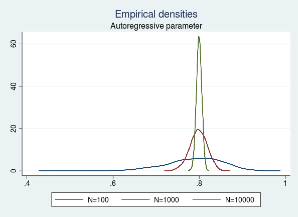
The empirical distribution for the estimated AR parameter is tighter around the true value of 0.8 for a sample size of 10,000 than that for a sample of size 100. The figure implies that as we keep increasing the sample size to \(\infty\), the AR estimate converges to the true value with probability 1. This implies that the QMLE is consistent.

Asymptotic normality

If \(\hat{\theta}_{\textrm{QMLE}}\) is a consistent estimator of the true value \(\theta\), then \(\sqrt{T}(\hat{\theta}_{\textrm{QMLE}}-\theta)\) converges in distribution to \(N(0,V)\) as \(T\) approaches \(\infty\) (White 1982). Assuming I have an infinite number of observations, the robust variance estimator provides a good approximation to the true variance. In this case, I obtain the "true" variance for the recentered and rescaled AR parameter to be 0.42 by using the robust variance estimator on a 10-million observation sample.

Let's look at the recentered and rescaled version of the empirical distributions of the AR parameters obtained for different sample sizes. I plot all the empirical distributions along with the "true" N(0,0.42) distribution for comparison.

. generate double ar_t100n = sqrt(100)*(ar_t100 - 0.8)

. generate double ar_t1000n = sqrt(1000)*(ar_t1000 - 0.8)

. generate double ar_t10000n = sqrt(10000)*(ar_t10000 - 0.8)

. kdensity ar_t100n, n(5000) generate(x_100n f_100n) kernel(gaussian) nograph

. label variable f_100n "N=100"

. kdensity ar_t1000n, n(5000) generate(x_1000n f_1000n) kernel(gaussian) 
> nograph

. label variable f_1000n "N=1000"

. kdensity ar_t10000n, n(5000) generate(x_10000n f_10000n) kernel(gaussian) 
> nograph

. label variable f_10000n "N=10000"

twoway (line f_100n x_100n) (line f_1000n x_1000n) (line f_10000n x_10000n) (4
> function normalden(x, sqrt(0.42)), range(-4 4)), legend( label(4 "Normal(0, 0
> .42)") cols(3)) title("Empirical densities") subtitle("Recentered and rescale
> d estimator and a N(0,0.42)")

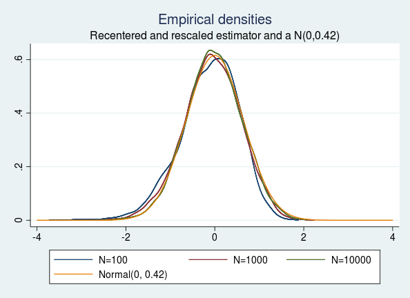
We see that the empirical densities of the recentered and rescaled estimators are indistinguishable from the density of a normal distribution with mean 0 and variance 0.42, as predicted by the theory.

Estimating rejection rates

I also assess the estimated standard error and asymptotic normality of the QMLE by checking the rejection rates. The Wald tests depend on the asymptotic normality of the estimate and a consistent estimate of the standard error. Summarizing the mean of the rejection rates of the estimated ARMA(1,1) for all sample sizes yields the following table.

. mean rr_ar* rr_ma*

Mean estimation                   Number of obs   =      5,000

--------------------------------------------------------------
             |       Mean   Std. Err.     [95% Conf. Interval]
-------------+------------------------------------------------
  rr_ar_t100 |       .069   .0035847      .0619723    .0760277
 rr_ar_t1000 |      .0578   .0033006      .0513294    .0642706
rr_ar_t10000 |      .0462    .002969      .0403795    .0520205
  rr_ma_t100 |      .0982   .0042089      .0899487    .1064513
 rr_ma_t1000 |       .056   .0032519      .0496248    .0623752
rr_ma_t10000 |       .048   .0030234      .0420728    .0539272
--------------------------------------------------------------

The rejection rates for the AR and MA parameters are large compared with the nominal size of 5% for a sample size of 100. As I increase the sample size, the rejection rate gets closer to the nominal size. This implies that the robust variance estimator yields a good coverage of the Wald test in large samples.

Conclusion

I used MCS to verify the consistency and asymptotic normality of the QMLE of an ARMA(1,1) model. I estimated the rejection rates for the AR and MA parameters using MCS and also verified that the robust variance estimator consistently estimates the true variance of the QMLE in large samples.

Appendix

MCS for a sample size of 1,000

. local T = 1000

. quietly postfile armasim ar_t1000 ma_t1000 rr_ar_t1000 rr_ma_t1000 using 
> t1000, replace

. forvalues i=1/`MC' {
  2.         quietly drop _all
  3.         local obs = `T' + 100
  4.         quietly set obs `obs'
  5.         quietly generate time = _n
  6.         quietly tsset time
  7. /*Generate data*/
.         quietly generate eps = rchi2(1)-1
  8.         quietly generate y = rnormal(0,1) in 1
  9.         quietly replace y = 0.8*l.y + eps + 0.5*l.eps in 2/l
 10.         quietly drop in 1/100
 11. /*Estimate*/
.         quietly arima y, ar(1) ma(1) nocons vce(robust)
 12.         quietly test _b[ARMA:l.ar]=0.8
 13.         local r_ar = (r(p)<0.05)
 14.         quietly test _b[ARMA:l.ma]=0.5
 15.         local r_ma = (r(p)<0.05)
 16.         post armasim (_b[ARMA:l.ar]) (_b[ARMA:l.ma]) (`r_ar') (`r_ma')
 17. }

. postclose armasim

MCS for a sample size of 10,000

. local T = 10000

. quietly postfile armasim ar_t10000 ma_t10000 rr_ar_t10000 rr_ma_t10000 using
> t10000, replace

. forvalues i=1/`MC' {
  2.         quietly drop _all
  3.         local obs = `T' + 100
  4.         quietly set obs `obs'
  5.         quietly generate time = _n
  6.         quietly tsset time
  7. /*Generate data*/
.         quietly generate eps = rchi2(1)-1
  8.         quietly generate y = rnormal(0,1) in 1
  9.         quietly replace y = 0.8*l.y + eps + 0.5*l.eps in 2/l
 10.         quietly drop in 1/100
 11. /*Estimate*/
.         quietly arima y, ar(1) ma(1) nocons vce(robust)
 12.         quietly test _b[ARMA:l.ar]=0.8
 13.         local r_ar = (r(p)<0.05)
 14.         quietly test _b[ARMA:l.ma]=0.5
 15.         local r_ma = (r(p)<0.05)
 16.         post armasim (_b[ARMA:l.ar]) (_b[ARMA:l.ma]) (`r_ar') (`r_ma')
 17. }

. postclose armasim

References

White, H. L., Jr. 1982. Maximum likelihood estimation of misspecified models. Econometrica 50: 1–25.

Yao, Q., and P. J. Brockwell. 2006. Gaussian maximum likelihood estimation for ARMA models I: time series. Journal of Time Series Analysis 27: 857–875.