A simulation-based explanation of consistency and asymptotic normality
Overview
In the frequentist approach to statistics, estimators are random variables because they are functions of random data. The finite-sample distributions of most of the estimators used in applied work are not known, because the estimators are complicated nonlinear functions of random data. These estimators have large-sample convergence properties that we use to approximate their behavior in finite samples.
Two key convergence properties are consistency and asymptotic normality. A consistent estimator gets arbitrarily close in probability to the true value. The distribution of an asymptotically normal estimator gets arbitrarily close to a normal distribution as the sample size increases. We use a recentered and rescaled version of this normal distribution to approximate the finite-sample distribution of our estimators.
I illustrate the meaning of consistency and asymptotic normality by Monte Carlo simulation (MCS). I use some of the Stata mechanics I discussed in Monte Carlo simulations using Stata.
Consistent estimator
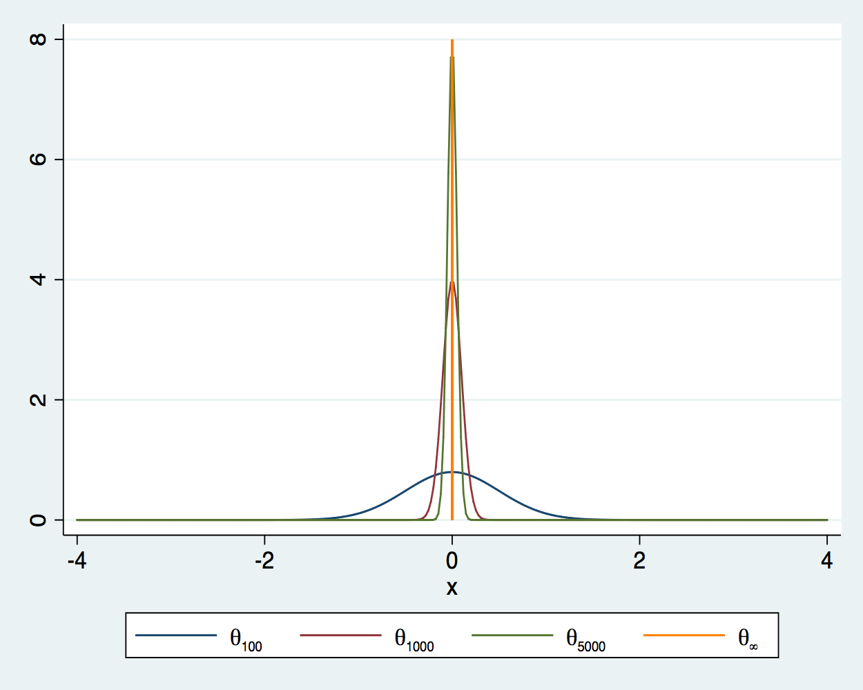
A consistent estimator gets arbitrarily close in probability to the true value as you increase the sample size. In other words, the probability that a consistent estimator is outside a neighborhood of the true value goes to zero as the sample size increases. Figure 1 illustrates this convergence for an estimator \(\theta\) at sample sizes 100, 1,000, and 5,000, when the true value is 0. As the sample size increases, the density is more tightly distributed around the true value. As the sample size becomes infinite, the density collapses to a spike at the true value.
Figure 1: Densities of an estimator for sample sizes 100, 1,000, 5,000, and \(\infty\)
I now illustrate that the sample average is a consistent estimator for the mean of an independently and identically distributed (i.i.d.) random variable with a finite mean and a finite variance. In this example, the data are i.i.d. draws from a \(\chi^2\) distribution with 1 degree of freedom. The true value is 1, because the mean of a \(\chi^2(1)\) is 1.
Code block 1 implements an MCS of the sample average for the mean from samples of size 1,000 of i.i.d. \(\chi^2(1)\) variates.
clear all
set seed 12345
postfile sim m1000 using sim1000, replace

forvalues i = 1/1000 {
        quietly capture drop y
        quietly set obs 1000
        quietly generate y = rchi2(1)
        quietly summarize y
        quietly post sim  (r(mean))
}
postclose sim
Line 1 clears Stata, and line 2 sets the seed of the random number generator. Line 3 uses postfile to create a place in memory named sim, in which I store observations on the variable m1000, which will be the new dataset sim1000. Note that the keyword using separates the name of the new variable from the name of the new dataset. The replace option specifies that sim1000.dta be replaced, if it already exists.
Lines 5 and 11 use forvalues to repeat the code in lines 6–10 1,000 times. Each time through the forvalues loop, line 6 drops y, line 7 sets the number of observations to 1,000, line 8 generates a sample of size 1,000 of i.i.d. \(\chi^2(1)\) variates, line 9 estimates the mean of y in this sample, and line 10 uses post to store the estimated mean in what will be the new variable m1000. Line 12 writes everything stored in sim to the new dataset sim100.dta. See Monte Carlo simulations using Stata for more details about using post to implement an MCS in Stata.
In example 1, I run mean1000.do and then summarize the results.
Example 1: Estimating the mean from a sample of size 1,000
. do mean1000

. clear all

. set seed 12345

. postfile sim m1000 using sim1000, replace

.
. forvalues i = 1/1000 {
  2.         quietly capture drop y
  3.         quietly set obs 1000
  4.         quietly generate y = rchi2(1)
  5.         quietly summarize y
  6.         quietly post sim  (r(mean))
  7. }

. postclose sim

.
.
end of do-file

. use sim1000, clear

. summarize m1000

    Variable |        Obs        Mean    Std. Dev.       Min        Max
-------------+---------------------------------------------------------
       m1000 |      1,000     1.00017    .0442332   .8480308   1.127382
The mean of the 1,000 estimates is close to 1. The standard deviation of the 1,000 estimates is 0.0442, which measures how tightly the estimator is distributed around the true value of 1.
Code block 2 contains mean100000.do, which implements the analogous MCS with
a sample size of 100,000.
clear all
// no seed, just keep drawing
postfile sim m100000 using sim100000, replace

forvalues i = 1/1000 {
        quietly capture drop y
        quietly set obs 100000
        quietly generate y = rchi2(1)
        quietly summarize y
        quietly post sim  (r(mean))
}
postclose sim
Example 2 runs mean100000.do and summarizes the results.
Example 2: Estimating the mean from a sample of size 100,000
. do mean100000

. clear all

. // no seed, just keep drawing
. postfile sim m100000 using sim100000, replace

.
. forvalues i = 1/1000 {
  2.         quietly capture drop y
  3.         quietly set obs 100000
  4.         quietly generate y = rchi2(1)
  5.         quietly summarize y
  6.         quietly post sim  (r(mean))
  7. }

. postclose sim

.
.
end of do-file

. use sim100000, clear

. summarize m100000

    Variable |        Obs        Mean    Std. Dev.       Min        Max
-------------+---------------------------------------------------------
     m100000 |      1,000    1.000008    .0043458   .9837129   1.012335
The standard deviation of 0.0043 indicates that the distribution of the estimator with a sample size 100,000 is much more tightly distributed around the true value of 1 than the estimator with a sample size of 1,000.
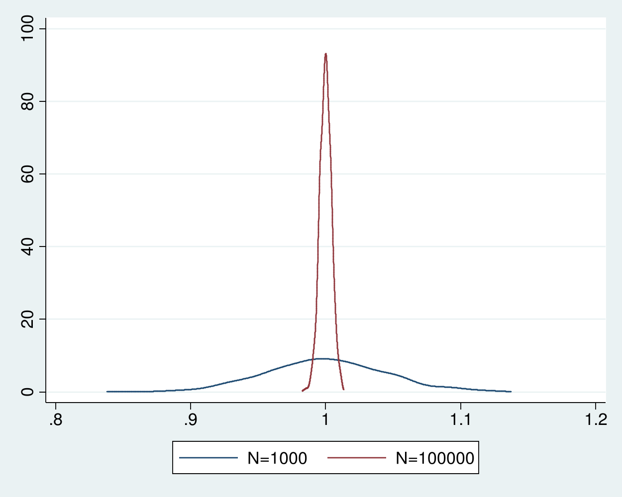
Example 3 merges the two datasets of estimates and plots the densities of the estimator for the two sample sizes in figure 2. The distribution of the estimator for the sample size of 100,000 is much tighter around 1 than the estimator for the sample size of 1,000.
Example 3: Densities of sample-average estimator for 1,000 and 100,000
. merge 1:1 _n using sim1000

    Result                           # of obs.
    -----------------------------------------
    not matched                             0
    matched                             1,000  (_merge==3)
    -----------------------------------------

. kdensity m1000, n(500) generate(x_1000 f_1000) kernel(gaussian) nograph

. label variable f_1000 "N=1000"

. kdensity m100000, n(500) generate(x_100000 f_100000) kernel(gaussian) nograph

. label variable f_100000 "N=100000"

. graph twoway (line f_1000 x_1000) (line f_100000 x_100000)
Figure 2: Densities of the sample-average estimator for sample sizes 1,000 and 100,000
The sample average is a consistent estimator for the mean of an i.i.d. \(\chi^2(1)\) random variable because a weak law of large numbers applies. This theorem specifies that the sample average converges in probability to the true mean if the data are i.i.d., the mean is finite, and the variance is finite. Other versions of this theorem weaken the i.i.d. assumption or the moment assumptions, see Cameron and Trivedi (2005, sec. A.3), Wasserman (2003, sec. 5.3), and Wooldridge (2010, 41–42) for details.
Asymptotic normality
So the good news is that distribution of a consistent estimator is arbitrarily tight around the true value. The bad news is the distribution of the estimator changes with the sample size, as illustrated in figures 1 and 2.
If I knew the distribution of my estimator for every sample size, I could use it to perform inference using this finite-sample distribution, also known as the exact distribution. But the finite-sample distribution of most of the estimators used in applied research is unknown. Fortunately, the distributions of a recentered and rescaled version of these estimators gets arbitrarily close to a normal distribution as the sample size increases. Estimators for which a recentered and rescaled version converges to a normal distribution are said to be asymptotically normal. We use this large-sample distribution to approximate the finite-sample distribution of the estimator.
Figure 2 shows that the distribution of the sample average becomes increasingly tight around the true value as the sample size increases. Instead of looking at the distribution of the estimator \(\widehat{\theta}_N\) for sample size \(N\), let’s look at the distribution of \(\sqrt{N}(\widehat{\theta}_N – \theta_0)\), where \(\theta_0\) is the true value for which \(\widehat{\theta}_N\) is consistent.
Example 4 estimates the densities of the recentered and rescaled estimators, which are shown in figure 3.
Example 4: Densities of the recentered and rescaled estimator
. generate double m1000n   =   sqrt(1000)*(m1000   - 1)

. generate double m100000n = sqrt(100000)*(m100000 - 1)

. kdensity m1000n, n(500) generate(x_1000n f_1000n) kernel(gaussian) nograph

. label variable f_1000n "N=1000"

. kdensity m100000n, n(500) generate(x_100000n f_100000n) kernel(gaussian) ///
>       nograph

. label variable f_100000n "N=100000"

. graph twoway (line f_1000n x_1000n) (line f_100000n x_100000n)
Figure 3: Densities of the recentered and rescaled estimator for sample sizes 1,000 and 100,000
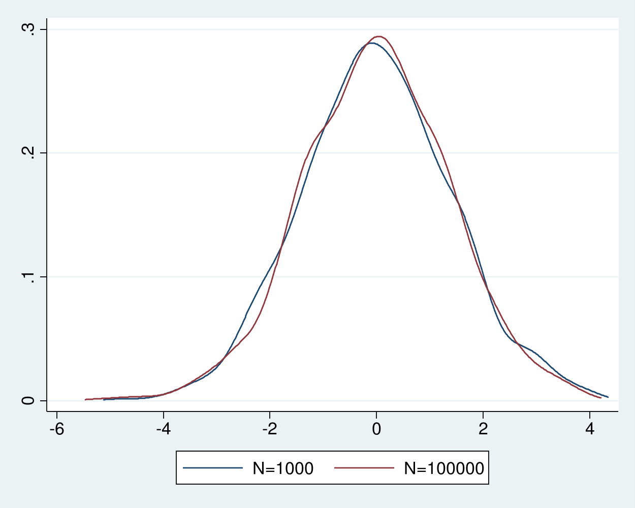
The densities of the recentered and rescaled estimators in figure 3 are indistinguishable from each and look close to a normal density. The Lindberg–Levy central limit theorem guarantees that the distribution of the recentered and rescaled sample average of i.i.d. random variables with finite mean \(\mu\) and finite variance \(\sigma^2\) gets arbitrarily closer to a normal distribution with mean 0 and variance \(\sigma^2\) as the sample size increases. In other words, the distribution of \(\sqrt{N}(\widehat{\theta}_N-\mu)\) gets arbitrarily close to a \(N(0,\sigma^2)\) distribution as \(\rightarrow\infty\), where \(\widehat{\theta}_N=1/N\sum_{i=1}^N y_i\) and \(y_i\) are realizations of the i.i.d. random variable. This convergence in distribution justifies our use of the distribution \(\widehat{\theta}_N\sim N(\mu,\frac{\sigma^2}{N})\) in practice.
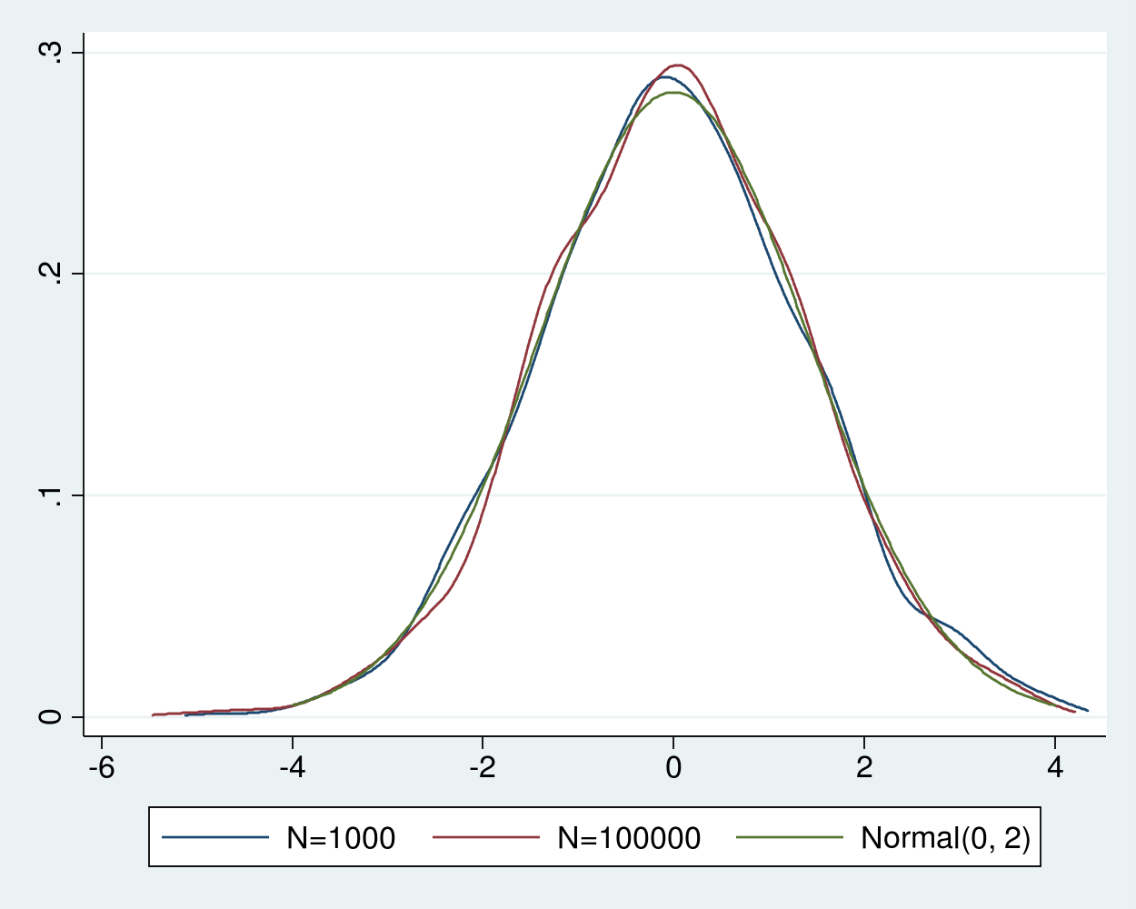
Given that \(\sigma^2=2\) for the \(\chi^2(1)\) distribution, in example 5, we add a plot of a normal density with mean 0 and variance 2 for comparison.
Example 5: Densities of the recentered and rescaled estimator
. twoway (line f_1000n x_1000n)                        ///
>        (line f_100000n x_100000n)                    ///
>        (function normalden(x, sqrt(2)), range(-4 4)) ///
>        ,legend( label(3 "Normal(0, 2)") cols(3))
We see that the densities of recentered and rescaled estimators are indistinguishable from the density of a normal distribution with mean 0 and variance 2, as predicted by the theory.
Figure 4: Densities of the recentered and rescaled estimates and a Normal(0,2)
Other versions of the central limit theorem weaken the i.i.d. assumption or the moment assumptions, see Cameron and Trivedi (2005, sec. A.3), Wasserman (2003, sec. 5.3), and Wooldridge (2010, 41–42) for details.
Done and undone
I used MCS to illustrate that the sample average is consistent and asymptotically normal for data drawn from an i.i.d. process with finite mean and variance.
Many method-of-moments estimators, maximum likelihood estimators, and M-estimators are consistent and asymptotically normal under assumptions about the true data-generating process and the estimators themselves. See Cameron and Trivedi (2005, sec. 5.3), Newey and McFadden (1994), Wasserman (2003, chap. 9), and Wooldridge (2010, chap. 12) for discussions.
Cameron, A. C., and P. K. Trivedi. 2005. Microeconometrics: Methods and Applications. Cambridge: Cambridge University Press.
Newey, W. K., and D. McFadden. 1994. Large sample estimation and hypothesis testing. In Handbook of Econometrics, ed. R. F. Engle and D. McFadden, vol. 4, 2111–2245. Amsterdam: Elsevier.
Wasserman, L. A. 2003. All of Statistics: A Concise Course in Statistical Inference. New York: Springer.
Wooldridge, J. M. 2010. Econometric Analysis of Cross Section and Panel Data. 2nd ed. Cambridge, Massachusetts: MIT Press.