\(\newcommand{\Eb}{{\bf E}}
\newcommand{\xb}{{\bf x}}
\newcommand{\betab}{\boldsymbol{\beta}}\)Differences in conditional probabilities and ratios of odds are two common measures of the effect of a covariate in binary-outcome models. I show how these measures differ in terms of conditional-on-covariate effects versus population-parameter effects.

Difference in graduation probabilities

I have simulated data on whether a student graduates in 4 years (graduate) for each of 1,000 students that entered an imaginary university in the same year. Before starting their first year, each student took a short course that taught study techniques and new material; iexam records each student’s grade on the final for this course. I am interested in the effect of the math and verbal SAT score sat on the probability that graduate=1 when I also condition on high-school grade-point average hgpa and iexam. I include an interaction term it=iexam/(hgpa^2) in the regression to allow for the possibility that iexam has a smaller effect for students with a higher hgpa. You can download the data by clicking on effectsb.dta.

Below I estimate the parameters of a logistic model that specifies the probability of graduation conditional on values of hgpa, sat, and iexam. (From here on, graduation probability is short for four-year graduation probability.)

Example 1: Logistic model for graduation probability condition on hgpa, sat, and iexam

. logit grad hgpa sat iexam it

Iteration 0:   log likelihood = -692.80914
Iteration 1:   log likelihood = -404.97166
Iteration 2:   log likelihood = -404.75089
Iteration 3:   log likelihood = -404.75078
Iteration 4:   log likelihood = -404.75078

Logistic regression                             Number of obs     =      1,000
                                                LR chi2(4)        =     576.12
                                                Prob > chi2       =     0.0000
Log likelihood = -404.75078                     Pseudo R2         =     0.4158

------------------------------------------------------------------------------
        grad |      Coef.   Std. Err.      z    P>|z|     [95% Conf. Interval]
-------------+----------------------------------------------------------------
        hgpa |   2.347051   .3975215     5.90   0.000     1.567923    3.126178
         sat |   1.790551   .1353122    13.23   0.000     1.525344    2.055758
       iexam |   1.447134   .1322484    10.94   0.000     1.187932    1.706336
          it |   1.713286   .7261668     2.36   0.018     .2900249    3.136546
       _cons |  -46.82946   3.168635   -14.78   0.000    -53.03987   -40.61905
------------------------------------------------------------------------------

The estimates imply that

\begin{align*}
\widehat{\bf Pr}[{\bf graduate=1}&| {\bf hgpa}, {\bf sat}, {\bf iexam}] \\
& = {\bf F}\left[
2.35{\bf hgpa} + 1.79 {\bf sat} + 1.45 {\bf iexam}\right. \\
&\quad \left. + 1.71 {\bf iexam}/{(\bf hgpa^2)} – 46.83\right]
\end{align*}

where \({\bf F}(\xb\betab)=\exp(\xb\betab)/[1+\exp(\xb\betab)]\) is the logistic distribution and \(\widehat{\bf Pr}[{\bf graduate=1}| {\bf hgpa}, {\bf sat}, {\bf iexam}]\) denotes the estimated conditional probability function.

Suppose that I am a researcher who wants to know the effect of getting a 1400 instead of a 1300 on the SAT on the conditional graduation probability. Because sat is measured in hundreds of points, the effect is estimated to be

\begin{align*}
\widehat{\bf Pr}&[{\bf graduate=1}|{\bf sat}=14, {\bf hgpa}, {\bf iexam}] \\
&\hspace{1cm}
-\widehat{\bf Pr}[{\bf graduate=1}|{\bf sat}=13, {\bf hgpa}, {\bf iexam}] \\
& = {\bf F}\left[
2.35{\bf hgpa} + 1.79 (14) + 1.45 {\bf iexam}
+ 1.71 {\bf iexam}/{(\bf hgpa^2)} – 46.83\right] \\
& \hspace{1cm} –
{\bf F}\left[
2.35{\bf hgpa} + 1.79 (13) + 1.45 {\bf iexam}
+ 1.71 {\bf iexam}/{(\bf hgpa^2)} – 46.83\right]
\end{align*}

The estimated effect of going from 1300 to 1400 on the SAT varies over the values of hgpa and iexam, because \({\bf F}()\) is nonlinear.

In example 2, I use predictnl to estimate these effects for each observation in the sample, and then I graph them.

Example 2: Estimated changes in graduation probabilities

. predictnl double diff =                                                    
>    logistic( _b[hgpa]*hgpa + _b[sat]*14 + _b[iexam]*iexam + _b[it]*it + _b[_cons]) 
>  - logistic( _b[hgpa]*hgpa + _b[sat]*13 + _b[iexam]*iexam + _b[it]*it + _b[_cons]) 
>    , ci(low up)
note: confidence intervals calculated using Z critical values

. sort diff

. generate ob = _n

. twoway (rarea low up ob) (scatter diff ob) , xlabels(none) xtitle("")
>    title("Conditional-on-covariate changes" "in graduation probabilities")

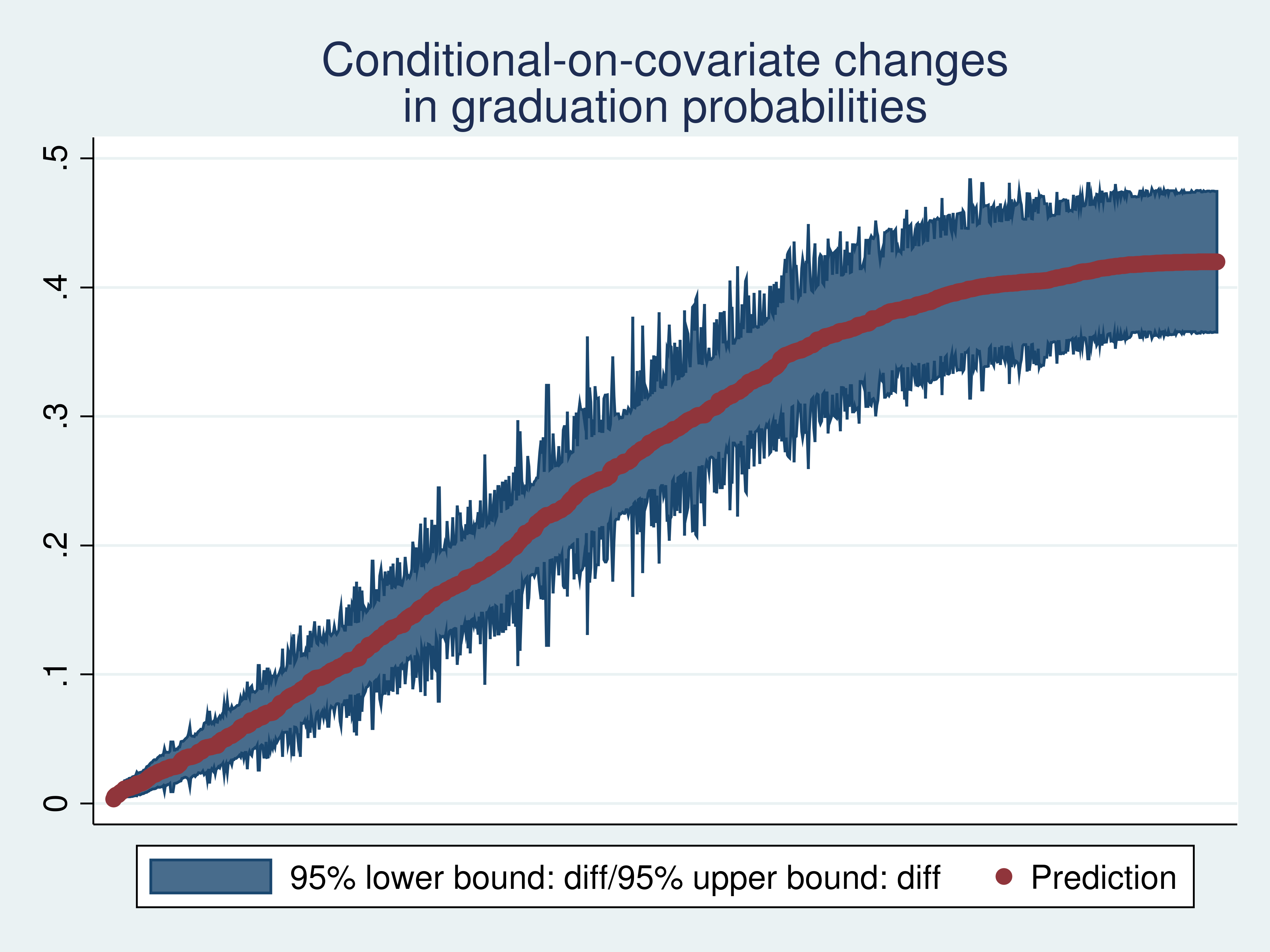
I see that the estimated differences in conditional graduation probabilities caused by going from 1300 to 1400 on the SAT range from close to 0 to more than 0.4 over the sample values of hgpa and iexam.

If I were a counselor advising specific students on the basis of their hgpa and iexam values, I would be interested in which students had effects near zero and in which students had effects greater than, say, 0.3. Methodologically, I would be interested in effects conditional on the covariates hgpa and iexam.

Instead, suppose I want to know “whether going from 1300 to 1400 on the SAT matters”, and I am thus interested in a single aggregate measure. In example 3, I use margins to estimate the mean of the conditional-on-covariate effects.

Example 3: Estimated mean of conditional changes in graduation probabilities

. margins , at(sat=(13 14)) contrast(atcontrast(r._at) nowald)

Contrasts of predictive margins
Model VCE    : OIM

Expression   : Pr(grad), predict()

1._at        : sat             =          13

2._at        : sat             =          14

--------------------------------------------------------------
             |            Delta-method
             |   Contrast   Std. Err.     [95% Conf. Interval]
-------------+------------------------------------------------
         _at |
   (2 vs 1)  |   .2576894   .0143522      .2295597    .2858192
--------------------------------------------------------------

The mean change in the conditional graduation probabilities caused by going from 1300 to 1400 on the SAT is estimated to be 0.22. It turns out that this mean change is the same as the difference in the probabilities that are only conditioned on the hypothesized sat values.

\begin{align*}
\Eb&\left[
\widehat{\bf Pr}[{\bf graduate=1}|{\bf sat}=14, {\bf hgpa}, {\bf iexam}] \right.
\\
&\quad
\left. -\widehat{\bf Pr}[{\bf graduate=1}|{\bf sat}=13, {\bf hgpa}, {\bf iexam}]
\right] \\
& =
\widehat{\bf Pr}[{\bf graduate=1}|{\bf sat}=14]
–
\widehat{\bf Pr}[{\bf graduate=1}|{\bf sat}=13]
\end{align*}

The mean of the changes in the conditional probabilities is a change in marginal probabilities. (\(\widehat{\bf Pr}[{\bf graduate=1}|{\bf sat}=14]\) and \(\widehat{\bf Pr}[{\bf graduate=1}|{\bf sat}=13]\) are conditional on the hypothesized sat values of interest and are marginal over hgpa and iexam.) The difference in the probabilities that condition only the values that define the “treatment” values is one of the population parameters that a potential-outcome approach would specify to be of interest.

Odds ratios

The odds of an event specifies how likely it is to occur, with higher values implying that the event is more likely. An odds ratio is the ratio of the odds of an event in one scenario to the odds of the same event under a different scenario. For example, I might be interested in the ratio of the graduation odds when a student has an SAT of 1400 to the graduation odds when a student has an SAT of 1300. A value greater than 1 implies that going from 1300 to 1400 has raised the graduation odds. A value less than 1 implies that going from 1300 to 1400 has lowered the graduation odds.

Because we used a logistic model for the conditional probability, the ratio of the odds of graduation conditional on sat=14, hgpa, and iexam to the odds of graduation conditional on sat=13, hgpa, and iexam is exp(_b[sat]), whose estimate we can obtain from
logit.

Example 4: Ratio of conditional-on-covariate graduation odds

. logit , or

Logistic regression                             Number of obs     =      1,000
                                                LR chi2(4)        =     576.12
                                                Prob > chi2       =     0.0000
Log likelihood = -404.75078                     Pseudo R2         =     0.4158

------------------------------------------------------------------------------
        grad | Odds Ratio   Std. Err.      z    P>|z|     [95% Conf. Interval]
-------------+----------------------------------------------------------------
        hgpa |   10.45469   4.155964     5.90   0.000     4.796674    22.78673
         sat |   5.992756   .8108931    13.23   0.000     4.596726    7.812761
       iexam |   4.250916   .5621767    10.94   0.000     3.280292    5.508743
          it |   5.547158   4.028162     2.36   0.018     1.336461    23.02421
       _cons |   4.59e-21   1.46e-20   -14.78   0.000     9.23e-24    2.29e-18
------------------------------------------------------------------------------

The conditional-on-covariate graduation odds are estimated to be 6 times higher for a student with a 1400 SAT than for a student with a 1300 SAT. This interpretation comes from some algebra that shows that

\begin{align*}
{\large \frac{
\frac{\widehat{\bf Pr}[{\bf graduate=1}|{\bf sat}=14, {\bf hgpa}, {\bf iexam}]}{
1-\widehat{\bf Pr}[{\bf graduate=1}|{\bf sat}=14, {\bf hgpa}, {\bf iexam}]}
}
{
\frac{\widehat{\bf Pr}[{\bf graduate=1}|{\bf sat}=13, {\bf hgpa}, {\bf iexam}]}{
1-\widehat{\bf Pr}[{\bf graduate=1}|{\bf sat}=13, {\bf hgpa}, {\bf iexam}]}
}}
=\exp\left({\bf \_b[sat]}\right)
\end{align*}

when

\begin{align*}
&\hspace{-.5em}\widehat{\bf Pr}[{\bf graduate=1}|{\bf sat}, {\bf hgpa}, {\bf iexam}] \\
&\hspace{-.5em}= {\small \frac{
{\bf exp(
\_b[hgpa] hgpa
+ \_b[sat] sat
+ \_b[iexam] iexam
+ \_b[it] it
+ \_b[\_cons]
)}
}
{
1 +
{\bf exp(
\_b[hgpa] hgpa
+ \_b[sat] sat
+ \_b[iexam] iexam
+ \_b[it] it
+ \_b[\_cons]
)}
}}
\end{align*}

In fact, a more general statement is possible. exp(_b[sat]) is the ratio of the conditional-on-covariate graduation odds for a student getting one more unit of sat to the conditional-on-covariate graduation odds for a student getting his or her current sat value.

Instead, I want to highlight that the logistic functional form makes this odds ratio a constant and that the ratio of conditional-on-covariate odds differs from the ratio of odds that condition only the hypothesized values.

Example 5 illustrates that the conditional-on-covariate odds ratio does not vary over the covariate patterns in the sample.

Example 5: Odds-ratio calculation

. generate sat_orig = sat

. replace sat  = 13
(999 real changes made)

. predict double pr0
(option pr assumed; Pr(grad))

. replace sat  = 14
(1,000 real changes made)

. predict double pr1
(option pr assumed; Pr(grad))

. replace sat  = sat_orig
(993 real changes made)

. generate orc = (pr1/(1-pr1))/(pr0/(1-pr0))

. summarize orc

    Variable |        Obs        Mean    Std. Dev.       Min        Max
-------------+---------------------------------------------------------
         orc |      1,000    5.992756           0   5.992756   5.992756

That the standard deviation is 0 highlights that the values are constant.

The ratio of the graduation odds that condition only on the hypothesized sat values differs from the mean of the ratios of graduation odds that condition on the hypothesized sat values and on hgpa and iexam. In contrast, the difference in the graduation probabilities that condition only on the hypothesized sat values is the same as the mean of the differences in graduation probabilities that condition on the hypothesized sat values and on hgpa and iexam.

Example 6 estimates the ratio of graduation odds that condition only on the hypothesized sat values.

Example 6: Odds ratio that conditions only on hypothesized sat values

. margins , at(sat=(13 14)) post

Predictive margins                              Number of obs     =      1,000
Model VCE    : OIM

Expression   : Pr(grad), predict()

1._at        : sat             =          13

2._at        : sat             =          14

------------------------------------------------------------------------------
             |            Delta-method
             |     Margin   Std. Err.      z    P>|z|     [95% Conf. Interval]
-------------+----------------------------------------------------------------
         _at |
          1  |   .2430499    .018038    13.47   0.000     .2076961    .2784036
          2  |   .5007393   .0133553    37.49   0.000     .4745634    .5269152
------------------------------------------------------------------------------

. nlcom (_b[2._at]/(1-_b[2._at]))/(_b[1._at]/(1-_b[1._at]))

       _nl_1:  (_b[2._at]/(1-_b[2._at]))/(_b[1._at]/(1-_b[1._at]))

------------------------------------------------------------------------------
             |      Coef.   Std. Err.      z    P>|z|     [95% Conf. Interval]
-------------+----------------------------------------------------------------
       _nl_1 |   3.123606   .2418127    12.92   0.000     2.649661     3.59755
------------------------------------------------------------------------------

Mathematically, this estimate implies that

\begin{align*}
\large{\frac{
\frac{\widehat{\bf Pr}[{\bf graduate=1}|{\bf sat}=14 ]}{
1-\widehat{\bf Pr}[{\bf graduate=1}|{\bf sat}=14 ]}
}
{
\frac{\widehat{\bf Pr}[{\bf graduate=1}|{\bf sat}=13 ]}{
1-\widehat{\bf Pr}[{\bf graduate=1}|{\bf sat}=13 ]}
}}
= 3.12
\end{align*}

The Delta-method standard error provides inference for the student in this sample as opposed to an unconditional standard error that provides inference for repeated sample from the population. (See Doctors versus policy analysts: Estimating the effect of interest for an example of how to obtain an unconditional standard error.)

The mean of a nonlinear function differs from a nonlinear function evaluated at the mean. Thus, the mean of conditional-on-covariate odds ratios differs from the odds ratio computed using means of conditional-on-covariate probabilities.

Which odds ratio is of interest depends on what you want to know. The conditional-on-covariate odds ratio is of interest when conditional-on-covariate comparisons are the goal, as is for the counselor discussed above. The ratio of the odds that condition only on hypothesized sat values is the population parameter that a potential-outcome approach would specify to be of interest.

Done and undone

In addition to discussing differences between conditional-on-covariate inference and population inference, I highlighted a difference between commonly used effect measures. The mean of differences in conditional-on-covariate probabilities is the same as a potential-outcome population parameter. In contrast, the mean of conditional-on-covariate odds ratios differs from the potential-outcome population parameter.