Doctors versus policy analysts: Estimating the effect of interest
\(\newcommand{\Eb}{{\bf E}}\)The change in a regression function that results from an everything-else-held-equal change in a covariate defines an effect of a covariate. I am interested in estimating and interpreting effects that are conditional on the covariates and averages of effects that vary over the individuals. I illustrate that these two types of effects answer different questions. Doctors, parents, and consultants frequently ask individuals for their covariate values to make individual-specific recommendations. Policy analysts use a population-averaged effect that accounts for the variation of the effects over the individuals.
Conditional on covariate effects after regress
I have simulated data on a college-success index (csuccess) on 1,000 students that entered an imaginary university in the same year. Before starting his or her first year, each student took a short course that taught study techniques and new material; iexam records each student grade on the final for this course. I am interested in the effect of the iexam score on the mean of csuccess when I also condition on high-school grade-point average hgpa and SAT score sat. I include an interaction term, it=iexam/(hgpa^2), in the regression to allow for the possibility that iexam has a smaller effect for students with a higher hgpa.
The regression below estimates the parameters of the conditional mean function that gives the mean of csuccess as a linear function of hgpa, sat, and iexam.
Example 1: mean of csuccess given hgpa, sat, and iexam
. regress csuccess hgpa sat iexam it, vce(robust)

Linear regression                             Number of obs     =      1,000
                                              F(4, 995)         =     384.34
                                              Prob > F          =     0.0000
                                              R-squared         =     0.5843
                                              Root MSE          =     1.3737

----------------------------------------------------------------------------
           |               Robust
  csuccess |      Coef.   Std. Err.      t    P>|t|     [95% Conf. Interval]
-----------+----------------------------------------------------------------
      hgpa |   .7030099    .178294     3.94   0.000     .3531344    1.052885
       sat |   1.011056   .0514416    19.65   0.000     .9101095    1.112002
     iexam |   .1779532   .0715848     2.49   0.013     .0374788    .3184276
        it |   5.450188   .3731664    14.61   0.000     4.717904    6.182471
     _cons |  -1.434994   1.059799    -1.35   0.176    -3.514692     .644704
----------------------------------------------------------------------------
The estimates imply that
\begin{align*}
\widehat{\Eb}[{\bf csuccess}| {\bf hgpa}, {\bf sat}, {\bf iexam}]
&=.70{\bf hgpa} + 1.01 {\bf sat} + 0.18 {\bf iexam} \\
&\quad + 5.45 {\bf iexam}/{(\bf hgpa^2)} – 1.43
\end{align*}
where \(\widehat{\Eb}[{\bf csuccess}| {\bf hgpa}, {\bf sat}, {\bf iexam}]\) denotes the estimated conditional mean function.
Because sat is measured in hundreds of points, the effect of a 100-point increase in sat is estimated to be
\begin{align*}
\widehat{\Eb}[{\bf csuccess}&| {\bf hgpa}, ({\bf sat}+1), {\bf iexam}]
–
\widehat{\Eb}[{\bf csuccess}| {\bf hgpa}, {\bf sat}, {\bf iexam}]\\
&=.70{\bf hgpa} + 1.01 ({\bf sat}+1) + 0.18 {\bf iexam} + 5.45 {\bf iexam}/{\bf hgpa^2} – 1.43 \\
&\hspace{1cm}- \left[.70{\bf hgpa} + 1.01 {\bf sat} + 0.18 {\bf iexam} + 5.45 {\bf iexam}/{\bf
hgpa^2} – 1.43 \right] \\
& = 1.01
\end{align*}
Note that the estimated effect of a 100-point increase in sat is a constant. The effect is also large, because the success index has a mean of 20.76 and a variance of 4.52; see example 2.
Example 2: Marginal distribution of college-success index
. summarize csuccess, detail

                          csuccess
-------------------------------------------------------------
      Percentiles      Smallest
 1%     16.93975       16.16835
 5%     17.71202       16.36104
10%     18.19191       16.53484       Obs               1,000
25%     19.25535        16.5457       Sum of Wgt.       1,000

50%     20.55144                      Mean           20.76273
                        Largest       Std. Dev.      2.126353
75%     21.98584       27.21029
90%     23.53014       27.33765       Variance       4.521379
95%     24.99978       27.78259       Skewness       .6362449
99%     26.71183       28.43473       Kurtosis        3.32826
Because iexam is measured in tens of points, the effect of a 10-point increase in the iexam is estimated to be
\begin{align*}
\widehat{\Eb}[{\bf csuccess}&| {\bf hgpa}, {\bf sat}, ({\bf iexam}+1)]
–
\widehat{\Eb}[{\bf csuccess}| {\bf hgpa}, {\bf sat}, {\bf iexam}] \\
& =.70{\bf hgpa} + 1.01 {\bf sat} + 0.18 ({\bf iexam}+1) + 5.45 ({\bf iexam}+1)/{(\bf hgpa^2)} – 1.43 \\
&\hspace{1cm}
-\left[.70{\bf hgpa} + 1.01 {\bf sat} + 0.18 {\bf iexam} + 5.45 {\bf iexam})/{(\bf hgpa^2)} – 1.43 \right] \\
& = .18 + 5.45 /{\bf hgpa^2}
\end{align*}
The effect varies with a student’s high-school grade-point average, so the conditional-on-covariate interpretation differs from the population-averaged interpretation. For example, suppose that I am a counselor who believes that only increases of 0.7 or more in csuccess matter, and a student with an hgpa of 4.0 asks me if a 10-point increase on the iexam will significantly affect his or her college success.
After using margins in example 3 to estimate the effect of a 10-point increase in iexam for someone with an hgpa=40, I tell the student “probably not”. (The estimated effect is 0.52, and the estimated upper bound of the 95% confidence interval is 0.64.)
Example 3: The effect of a 10-point increase in iexam when hgpa=4
. margins, expression(_b[iexam] + _b[it]/(hgpa^2)) at(hgpa=4)
Warning: expression() does not contain predict() or xb().

Predictive margins                            Number of obs     =      1,000
Model VCE    : Robust

Expression   : _b[iexam] + _b[it]/(hgpa^2)
at           : hgpa            =           4

----------------------------------------------------------------------------
           |            Delta-method
           |     Margin   Std. Err.      z    P>|z|     [95% Conf. Interval]
-----------+----------------------------------------------------------------
     _cons |     .51859   .0621809     8.34   0.000     .3967176    .6404623
----------------------------------------------------------------------------
After the student leaves, I run example 4 to estimate the effect of a 10-point increase in iexam when hgpa is 2, 2.5, 3, 3.5, and 4.
Example 4: The effect of a 10-point increase in iexam when hgpa is 2, 2.5, 3, 3.5, and 4
. margins, expression(_b[iexam] + _b[it]/(hgpa^2)) at(hgpa=(2 2.5 3 3.5 4))
Warning: expression() does not contain predict() or xb().

Predictive margins                            Number of obs     =      1,000
Model VCE    : Robust

Expression   : _b[iexam] + _b[it]/(hgpa^2)

1._at        : hgpa            =           2

2._at        : hgpa            =         2.5

3._at        : hgpa            =           3

4._at        : hgpa            =         3.5

5._at        : hgpa            =           4

----------------------------------------------------------------------------
           |            Delta-method
           |     Margin   Std. Err.      z    P>|z|     [95% Conf. Interval]
-----------+----------------------------------------------------------------
       _at |
        1  |     1.5405   .0813648    18.93   0.000     1.381028    1.699972
        2  |   1.049983   .0638473    16.45   0.000     .9248449    1.175122
        3  |   .7835297   .0603343    12.99   0.000     .6652765    .9017828
        4  |   .6228665   .0608185    10.24   0.000     .5036645    .7420685
        5  |     .51859   .0621809     8.34   0.000     .3967176    .6404623
----------------------------------------------------------------------------
I use marginsplot to further clarify these results.
Example 5: marginsplot
. marginsplot, yline(.7) ylabel(.5 .7 1 1.5 2)

  Variables that uniquely identify margins: hgpa
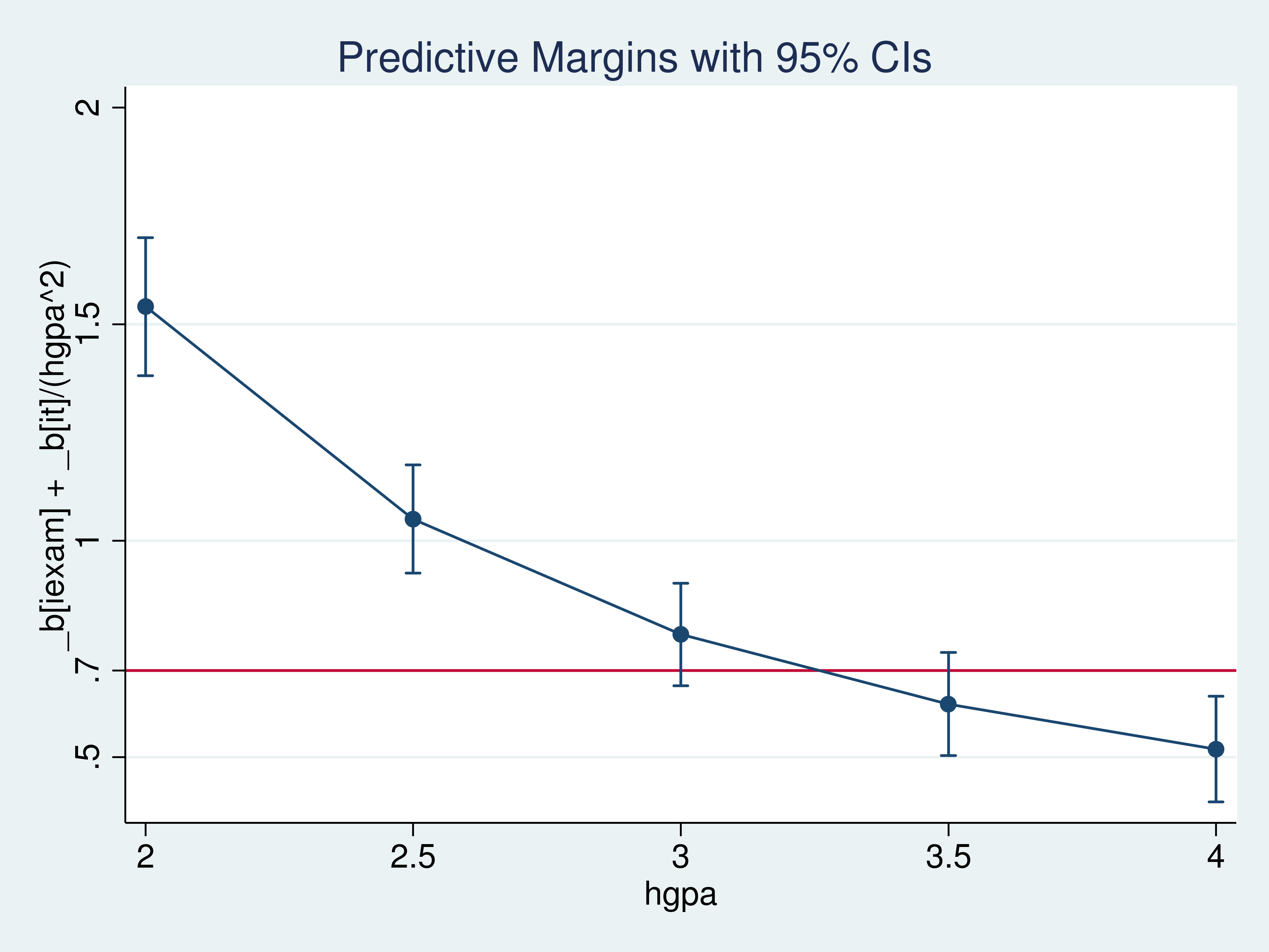
I could not rule out the possibility that a 10-point increase in iexam would cause an increase of 0.7 in the average csuccess for a student with an hgpa of 3.5.
Consider the case in which \(\Eb[y|x,{\bf z}]\) is my regression model for the outcome \(y\) as a function of \(x\), whose effect I want to estimate, and \({\bf z}\), which are other variables on which I condition. The regression function \(\Eb[y|x,{\bf z}]\) tells me the mean of \(y\) for given values of \(x\) and \({\bf z}\).
The difference between the mean of \(y\) given \(x_1\) and \({\bf z}\) and the mean of \(y\) given \(x_0\) and \({\bf z}\) is an effect of \(x\), and it is given by \(\Eb[y|x=x_1,{\bf z}] – \Eb[y|x=x_0,{\bf z}]\). This effect can vary with \({\bf z}\); it might be scientifically and statistically significant for some values of \({\bf z}\) and not for others.
Under the usual assumption of correct specification, I can estimate the parameters of \(\Eb[y|x,{\bf z}]\) using regress or another command. I can then use margins and marginsplot to estimate effects of \(x\). (I also frequently use lincom, nlcom, and predictnl to estimate effects of \(x\) for given \({\bf z}\) values.)
Population-averaged effects after regress
Returning to the example, instead of being a counselor, suppose that I am a university administrator who believes that assigning enough tutors to the course will raise each student’s iexam score by 10 points. I begin by using margins to estimate the average college-success score that is observed when each student gets his or her current iexam score and to estimate the average college-success score that would be observed when each student gets an extra 10 points on his or her iexam score.
Example 5: The average of csuccess with current iexam scores and when each student gets an extra 10 points
. margins, at(iexam = generate(iexam))
>         at(iexam = generate(iexam+1) it = generate((iexam+1)/(hgpa^2)))

Predictive margins                            Number of obs     =      1,000
Model VCE    : Robust

Expression   : Linear prediction, predict()

1._at        : iexam           = iexam

2._at        : iexam           = iexam+1
               it              = (iexam+1)/(hgpa^2)

----------------------------------------------------------------------------
           |            Delta-method
           |     Margin   Std. Err.      t    P>|t|     [95% Conf. Interval]
-----------+----------------------------------------------------------------
       _at |
        1  |   20.76273   .0434416   477.95   0.000     20.67748    20.84798
        2  |   21.48141   .0744306   288.61   0.000     21.33535    21.62747
----------------------------------------------------------------------------
Just to make sure that I understand what margins is doing, I compute the average of the predicted values when each student gets his or her current iexam score and when each student gets an extra 10 points on his or her iexam score.
Example 6: The average of csuccess with current iexam scores and when each student gets an extra 10 points (hand calculations)
. preserve

. predict double yhat0
(option xb assumed; fitted values)

. replace iexam       = iexam + 1
(1,000 real changes made)

. replace it          = (iexam)/(hgpa^2)
(1,000 real changes made)

. predict double yhat1
(option xb assumed; fitted values)

. summarize yhat0 yhat1

    Variable |      Obs        Mean    Std. Dev.       Min        Max
-------------+-------------------------------------------------------
       yhat0 |    1,000    20.76273    1.625351   17.33157   26.56351
       yhat1 |    1,000    21.48141    1.798292   17.82295   27.76324

. restore
As expected, the average of the predictions for yhat0 match those reported by margins for _at.1, and the average of the predictions for yhat1 match those reported by margins for _at.2.
Now that I understand what margins is doing, I use the contrast option to estimate the difference between the average of csuccess when each student gets an extra 10 points and the average of csuccess when each student gets his or her original score.
Example 7: The difference in the averages of csuccess when each student gets an extra 10 points and with current scores
. margins, at(iexam = generate(iexam))
>         at(iexam = generate(iexam+1) it = generate((iexam+1)/(hgpa^2)))
>         contrast(atcontrast(r._at) nowald)

Contrasts of predictive margins
Model VCE    : Robust

Expression   : Linear prediction, predict()

1._at        : iexam           = iexam

2._at        : iexam           = iexam+1
               it              = (iexam+1)/(hgpa^2)

--------------------------------------------------------------
             |            Delta-method
             |   Contrast   Std. Err.     [95% Conf. Interval]
-------------+------------------------------------------------
         _at |
   (2 vs 1)  |   .7186786   .0602891      .6003702     .836987
--------------------------------------------------------------
The standard error in example 7 is labeled as “Delta-method”, which means that it takes the covariate observations as fixed and accounts for the parameter estimation error. Holding the covariate observations as fixed gets me inference for this particular batch of students. I add the option vce(unconditional) in example 8, because I want inference for the population from which I can repeatedly draw samples of students.
Example 8: The difference in the averages of csuccess with an unconditional standard error
. margins, at(iexam = generate(iexam))
>         at(iexam = generate(iexam+1) it = generate((iexam+1)/(hgpa^2)))
>         contrast(atcontrast(r._at) nowald) vce(unconditional)

Contrasts of predictive margins

Expression   : Linear prediction, predict()

1._at        : iexam           = iexam

2._at        : iexam           = iexam+1
               it              = (iexam+1)/(hgpa^2)

--------------------------------------------------------------
             |            Unconditional
             |   Contrast   Std. Err.     [95% Conf. Interval]
-------------+------------------------------------------------
         _at |
   (2 vs 1)  |   .7186786   .0609148      .5991425    .8382148
--------------------------------------------------------------
In this case, the standard error for the sample effect reported in example 7 is about the same as the standard error for the population effect reported in example 8. With real data, the difference in these standard errors tends to be greater.
Recall the case in which \(\Eb[y|x,{\bf z}]\) is my regression model for the outcome \(y\) as a function of \(x\), whose effect I want to estimate, and \({\bf z}\), which are other variables on which I condition. The difference between the mean of \(y\) given \(x_1\) and the mean of \(y\) given \(x_0\) is an effect of \(x\) that has been averaged over the distribution of \({\bf z}\),
\[
\Eb[y|x=x_1] – \Eb[y|x=x_0] = \Eb_{\bf Z}\left[ \Eb[y|x=x_1,{\bf z}]\right] –
\Eb_{\bf Z}\left[ \Eb[y|x=x_0,{\bf z}]\right]
\]
Under the usual assumptions of correct specification, I can estimate the parameters of \(\Eb[y|x,{\bf z}]\) using regress or another command. I can then use margins and marginsplot to estimate a mean of these effects of \(x\). The sample must be representative, perhaps after weighting, in order for the estimated mean of the effects to converge to a population mean.
Done and undone
The change in a regression function that results from an everything-else-held-equal change in a covariate defines an effect of a covariate. I illustrated that when a covariate enters the regression function nonlinearly, the effect varies over covariate values, causing the conditional-on-covariate effect to differ from the population-averaged effect. I also showed how to estimate and interpret these conditional-on-covariate and population-averaged effects.