Quantile regression models a quantile of the outcome as a function of covariates. Applied researchers use quantile regressions because they allow the effect of a covariate to differ across conditional quantiles. For example, another year of education may have a large effect on a low conditional quantile of income but a much smaller effect on a high conditional quantile of income. Also, another pack-year of cigarettes may have a larger effect on a low conditional quantile of bronchial effectiveness than on a high conditional quantile of bronchial effectiveness.

I use simulated data to illustrate what the conditional quantile functions estimated by quantile regression are and what the estimable covariate effects are.

Simulated data to understand conditional quantiles

Suppose that each number between 0 and 1 corresponds to the fortune of an individual, or observational unit, in the population. In a sense, each number between 0 and 1 specifies the rank of an individual. For a given \(x\), a conditional quantile \(Q(\tau|x)\) maps a rank \(\tau\in[0,1]\) to an outcome \(y\). This mapping is essentially an inverse of the conditional distribution function. For each \(x\), a conditional distribution function \(F(y|x)\) maps an outcome \(y\) into a probability that must be between 0 and 1.

I drew simulated data from a Weibull distribution to illustrate what conditional quantiles are. The graph below contains a scatterplot of the outcome \(y\) against the covariate \(x\). I include plots of the conditional mean \(y\) given \(x\) (E[y|x]), the conditional 0.8 quantile of \(y\) given \(x\) (Q(0.8|x)), the conditional median of \(y\) given \(x\) (Q(0.5|x)), and the conditional 0.2 quantile of \(y\) given \(x\) (Q(0.2|x)).

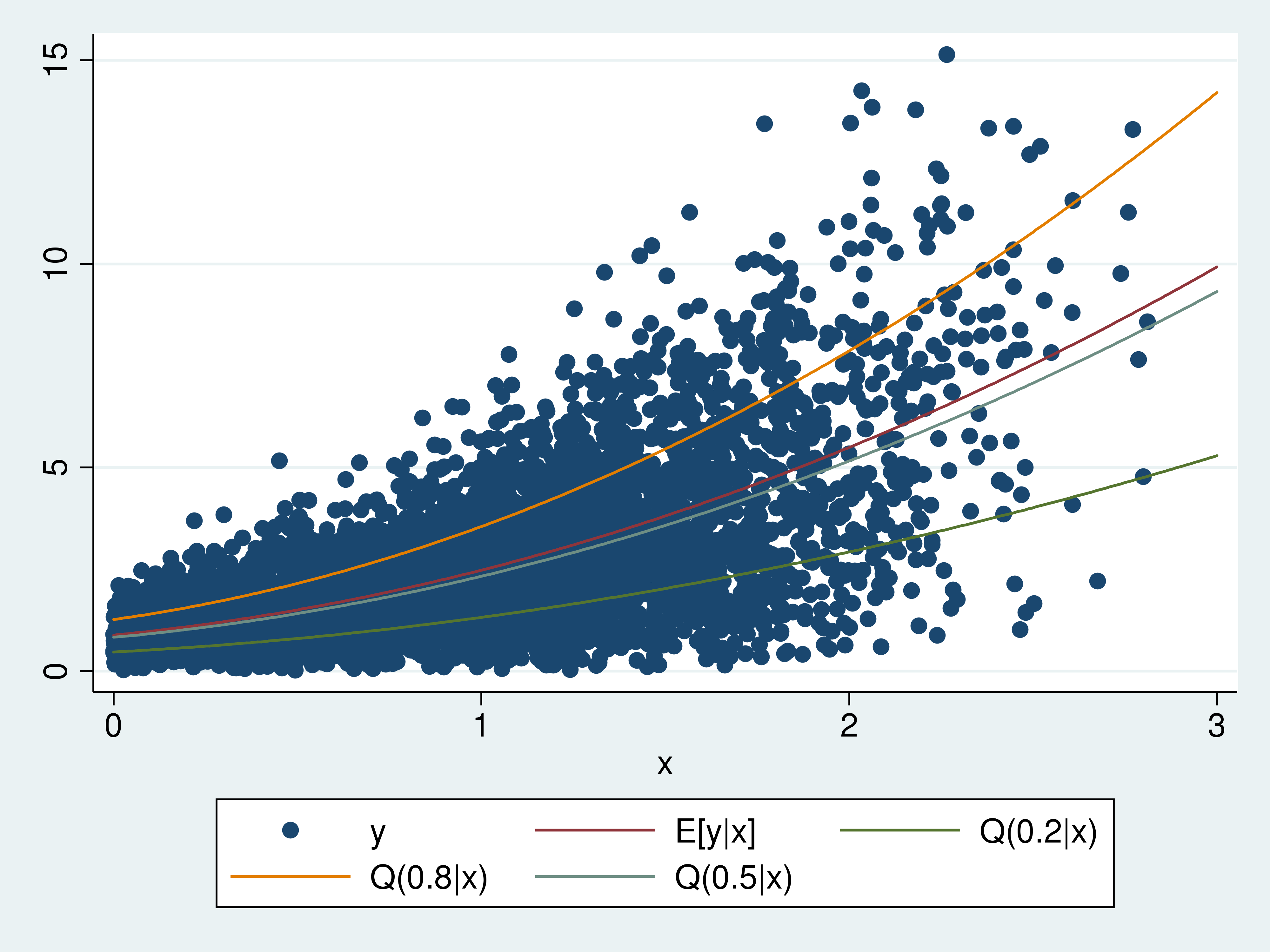
The Q(0.8|x) curve plots the outcome \(y\) corresponding to the rank of 0.8 for each \(x\). The Q(0.5|x) curve plots the outcome \(y\) corresponding to the rank of 0.5 for each \(x\). The Q(0.2|x) curve plots the outcome \(y\) corresponding to the rank of 0.2 for each \(x\). Q(0.8|x)>Q(0.5|x)>Q(0.2|x) for each \(x\) because \(0.8>0.5>0.2\).

The conditional mean and the conditional quantiles curve upward because I used a quadratic in \(x\) in the Weibull distribution of \(y\) given \(x\). The conditional mean is above the conditional median because the Weibull distribution has a long, thin right tail.

While the graph of the simulated data and the conditional quantiles provides some intuition, some technical details provide a deeper understanding. The functional form for the distribution of \(y\) given \(x\) from which I drew the data is

\begin{equation}
\label{F}\tag{1}
F(y|x)=1 -\exp\left[-\left(\frac{y}{
\beta_0 + \beta_1 x + \beta_2 x^2
}\right)^{\alpha}\right]
\end{equation}

The quantile function is the inverse distribution function for a continuous distribution. For quantile \(\tau\in[0,1]\), the conditional quantile function implied by the \(F(y|x)\) in \eqref{F} is

\begin{equation}
\label{Q}\tag{2}
Q(\tau|x) =
(\beta_0 + \beta_1 x + \beta_2 x^2)
\left[
-\ln(1-\tau)
\right]^{\frac{1}{\alpha}}
\end{equation}

For a specified value of \(x\), \(Q(\tau|x)\) produces the \(\tau\)(th) quantile of \(y\) conditional on \(x\).

I got \eqref{Q} by setting

$$
\tau=1 -\exp\left[-\left(\frac{y}{
\beta_0 + \beta_1 x + \beta_2 x^2
}\right)^{\alpha}\right]
$$

and solving for \(y\) as a function of \(\tau\). This inverse relationship is the foundation for the interpretation of the conditional quantile curves given above. For a given \(x\), \(F(y|x)\) maps \(y\) into where it ranks in \([0,1]\). For a given \(x\), \(Q(\tau|x)\) maps the rank \(\tau\) into the outcome \(y\).

Estimating conditional quantile functions

qreg estimates the parameters of conditional quantile functions. Like ordinary least squares, the conditional quantile functions are assumed to be linear combinations of covariates. Powers and interactions are accommodated using factor variables.

In example 1, I estimate \(\delta_0\), \(\delta_1\), and \(\delta_2\) in \(Q(0.2|x)= \delta_0 + \delta_1 x + \delta_2 x^2\).

Example 1: qreg for 0.2 conditional quantile

. use quantile1

. qreg y x c.x#c.x, quantile(0.2)
Iteration  1:  WLS sum of weighted deviations =  2549.6656

Iteration  1: sum of abs. weighted deviations =  2675.4783
Iteration  2: sum of abs. weighted deviations =  2382.9844
Iteration  3: sum of abs. weighted deviations =  2261.3777
Iteration  4: sum of abs. weighted deviations =  1855.4505
Iteration  5: sum of abs. weighted deviations =  1687.6014
Iteration  6: sum of abs. weighted deviations =  1664.1955
Iteration  7: sum of abs. weighted deviations =  1663.5237
Iteration  8: sum of abs. weighted deviations =  1661.7397
Iteration  9: sum of abs. weighted deviations =  1661.4886
Iteration 10: sum of abs. weighted deviations =   1661.485
Iteration 11: sum of abs. weighted deviations =  1661.4436
Iteration 12: sum of abs. weighted deviations =   1661.441
Iteration 13: sum of abs. weighted deviations =  1661.4379
Iteration 14: sum of abs. weighted deviations =  1661.4378

.2 Quantile regression                              Number of obs =      5,000
  Raw sum of deviations  1907.42 (about .95246261)
  Min sum of deviations 1661.438                    Pseudo R2     =     0.1290

------------------------------------------------------------------------------
           y |      Coef.   Std. Err.      t    P>|t|     [95% Conf. Interval]
-------------+----------------------------------------------------------------
           x |   .4528183   .1370586     3.30   0.001     .1841233    .7215133
             |
     c.x#c.x |   .3749397   .0625822     5.99   0.000     .2522511    .4976282
             |
       _cons |   .4922369   .0650939     7.56   0.000     .3646242    .6198496
------------------------------------------------------------------------------

You can download the data by clicking on this link quantile1.dta.

As reflected in the iteration log, qreg obtains its estimates by minimizing the sum of asymmetrically weighted absolute deviations; see Koenker and Bassett (1978), Cameron and Trivedi (2010, chap. 7.2.2), and Wooldridge (2010, chap. 12.10) for details. The output table presents point estimates and inference for the \(\delta_0\), \(\delta_1\), and \(\delta_2\) in \(Q(0.2|x)= \delta_0 + \delta_1 x + \delta_2 x^2\).

When I simulated the data, I set \(\beta_0=1\), \(\beta_1=1\), \(\beta_2=.8\), and \(\alpha=2\) in \eqref{F}. These values imply that the true values of \(\delta_0\), \(\delta_1\), and \(\delta_2\) are 0.47, 0.47, and 0.38, respectively. The estimated coefficients are close to their true values.

Comparing the estimated 0.2 conditional quantiles with the true function is another way of providing intuition for quantile regression. Example 2 computes the predictions and plots them on a graph that also contains a scatterplot of a subset of the data and a plot of the true 0.2 conditional quantile function.

Example 2: Estimated and true 0.2 conditional quantile functions

. predict xb0
(option xb assumed; fitted values)

. label variable xb0 "original predictions"

. sort x

. twoway (scatter y x if y<6)                                             
>  (function q20  = (1+x+0.8*x^2)*((-ln(1-0.2))^(1/2)) , range(0 3) )      
>  (line xb0 x)                                                           
>  , legend(label(2 "Q(0.2|x)")) legend(cols(3))

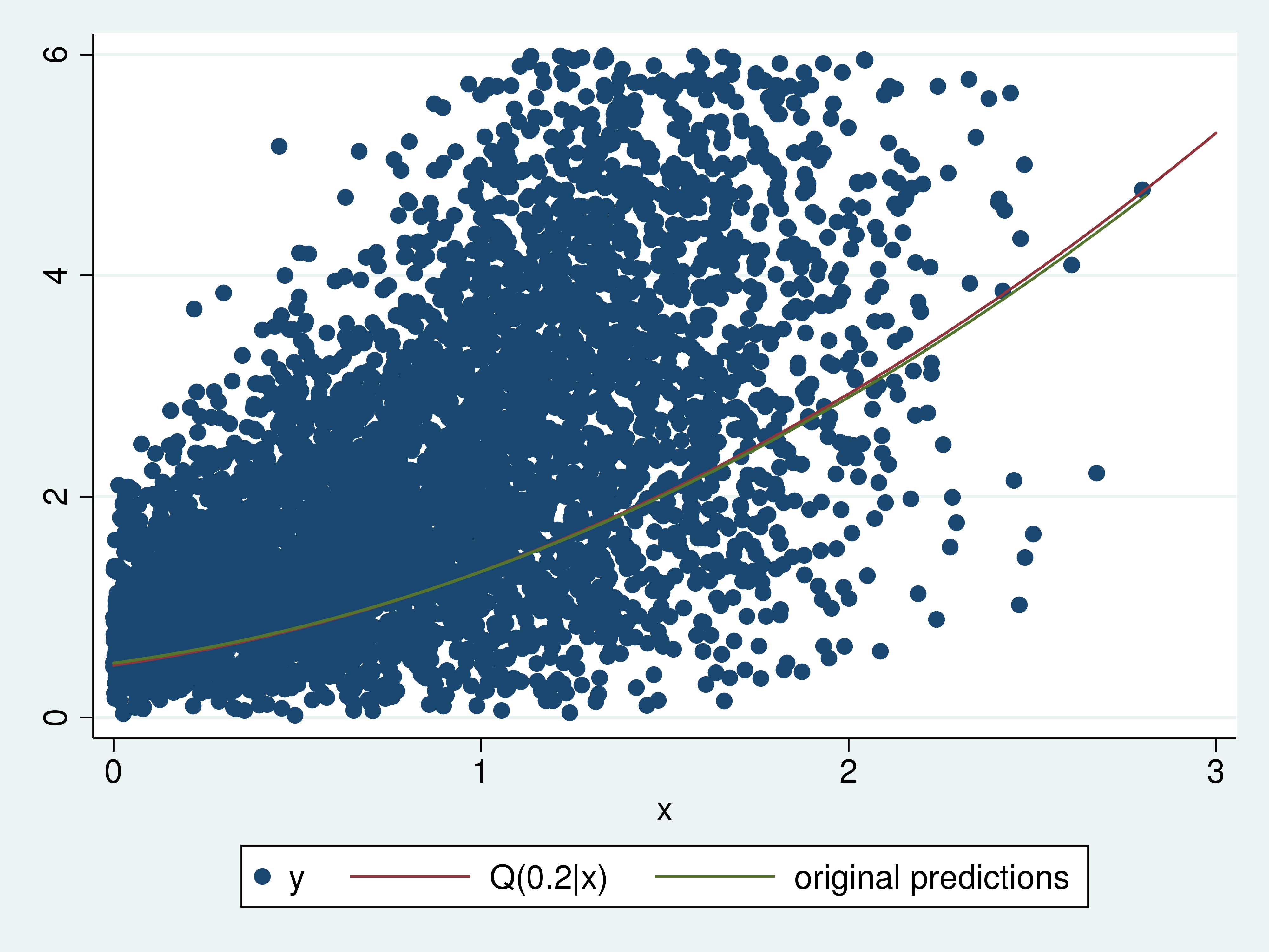
The estimated 0.2 conditional quantile function is very close to the true 0.2 conditional quantile function. In fact, I excluded larger observations from the scatterplot so that some difference in the curves is apparent.

Estimating covariate effects

The change in the \(\tau\)(th) conditional quantile function that results from a change in a covariate defines a covariate effect. For example, the difference in the 0.2 conditional quantile function that results from each unit getting an additional unit of \(x\) is \(Q(0.2|(x+1))-Q(0.2|x)\) is one such effect. Using the predictions computed in example 2, I compute and plot these estimated effects in example 3.

Example 3: Q(0.2|(x+1))-Q(0.2|x)

. generate orig = x

. replace x = x+1
(5,000 real changes made)

. predict xb1
(option xb assumed; fitted values)

. label variable xb1 "x=x+1 predictions"

. replace x = orig
(5,000 real changes made)

. generate effects = xb1 - xb0

. label variable effects "Q(0.2|(x+1)) - Q(0.2|x)"

. scatter effects x

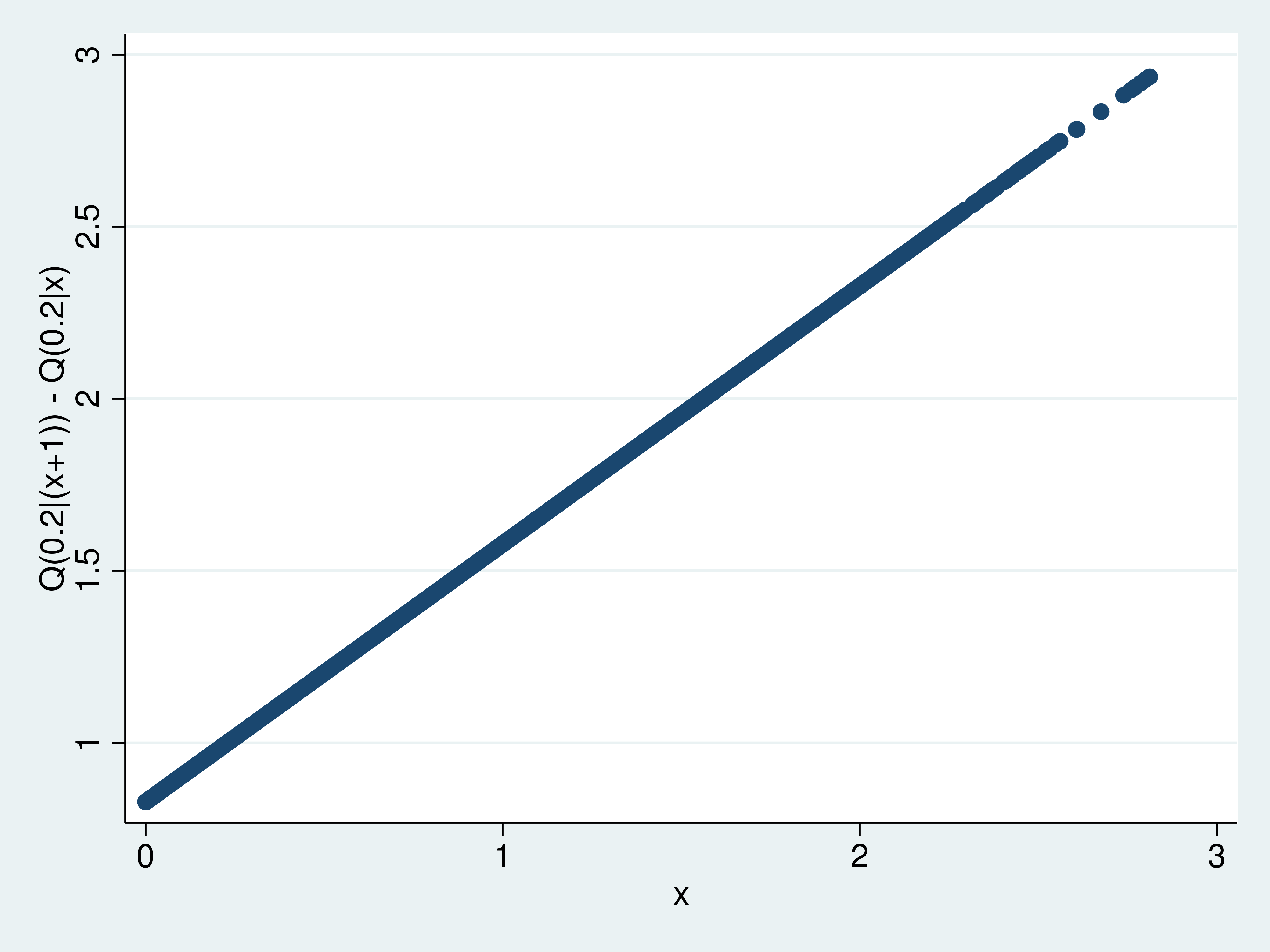
This graph shows how the effects vary over \(x\), but there is no information about how well these effects are estimated. predictnl estimates observation-level expressions of estimated parameters and produces pointwise confidence intervals. The expression for the effect of interest is

_b[x] + 2*_b[c.x#c.x]*x + _b[c.x#c.x]

because

_b[x]*(x+1) + _b[c.x#c.x]*(x+1)^2 + _b[_cons]
-(_b[x]*x + _b[c.x#c.x]*x^2 + _b[_cons])
= _b[x] + 2*_b[c.x#c.x]*x + _b[c.x#c.x]

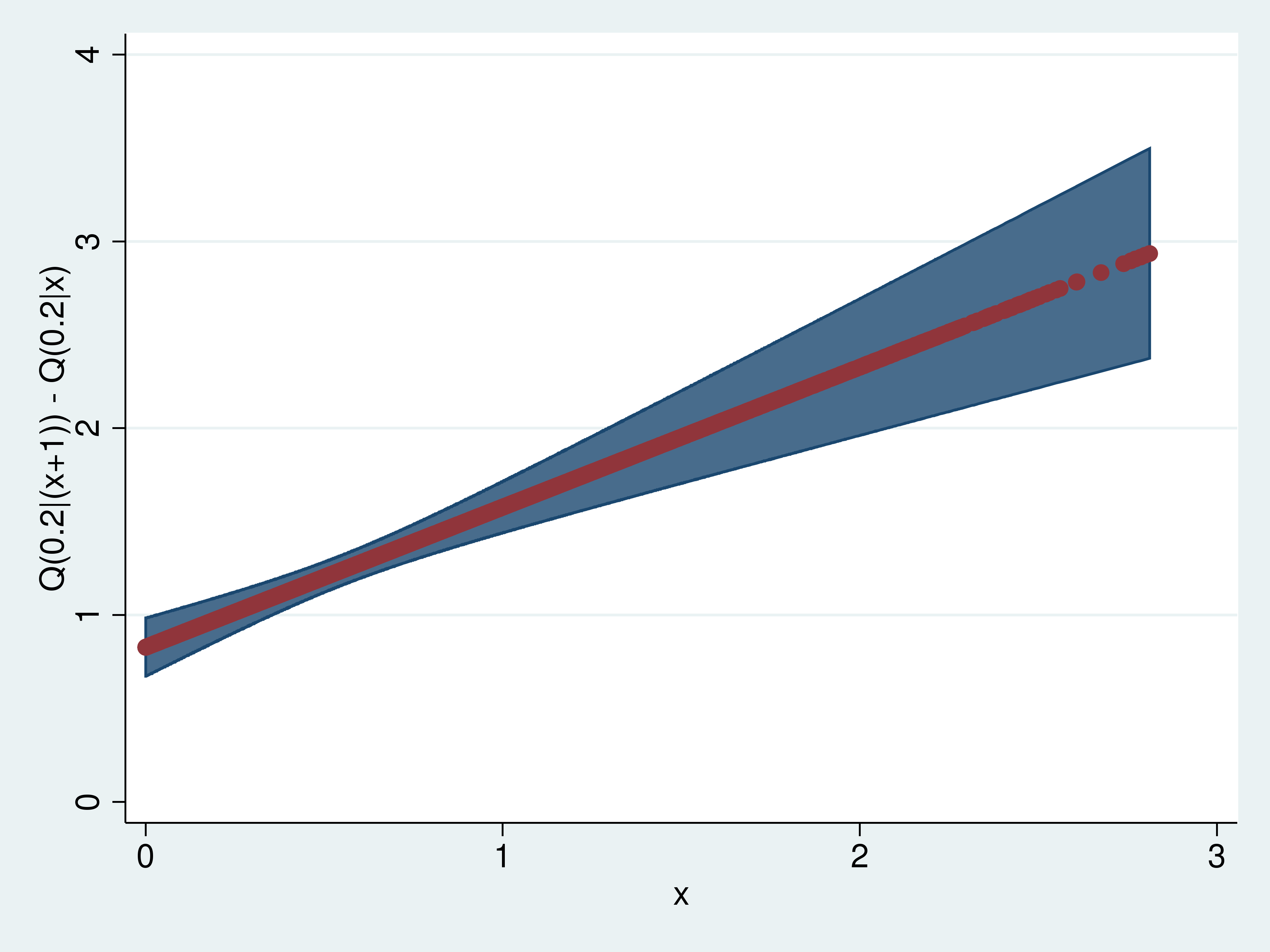
In example 4, I use predictnl to compute these effects and pointwise confidence intervals.

Example 4: predictnl estimates of Q(0.2|(x+1))-Q(0.2|x)

. predictnl effects2 = _b[x] + 2*_b[c.x#c.x]*x + _b[c.x#c.x], 
>         ci(low up)
note: confidence intervals calculated using Z critical values

. list effects effects2 in 1/5

     +---------------------+
     |  effects   effects2 |
     |---------------------|
  1. | .8279508   .8279508 |
  2. |  .828063   .8280631 |
  3. | .8281841   .8281842 |
  4. | .8283278   .8283277 |
  5. | .8286009   .8286009 |
     +---------------------+

. label variable effects2 "Q(0.2|(x+1)) - Q(0.2|x)"

. sort x

. twoway (rarea up low x) (scatter effects2 x),              
>         ytitle("Q(0.2|(x+1)) - Q(0.2|x)") legend(off)

I list the first five estimated effects to illustrate that the two computations yield the same results. Having illustrated this equivalence, I plot the effects with a confidence interval.

One of the reasons that researchers use quantile regression is that the effects can differ by quantile. The hypothesis is that the covariate effects differ for those dealt a low rank (quantile) than for those who are dealt a high rank (quantile). To compare the estimated effects of an additional unit of \(x\) on the 0.2 conditional quantile with these effects on the 0.8 conditional quantile, I begin by estimating the parameters of 0.8 conditional quantile function.

Example 5: qreg for 0.8 conditional quantile

. qreg y x c.x#c.x, quantile(.8)
Iteration  1:  WLS sum of weighted deviations =  2598.5922

Iteration  1: sum of abs. weighted deviations =  2602.1666
Iteration  2: sum of abs. weighted deviations =  2137.2076
Iteration  3: sum of abs. weighted deviations =  2060.0299
Iteration  4: sum of abs. weighted deviations =  2023.7347
Iteration  5: sum of abs. weighted deviations =  2019.0775
Iteration  6: sum of abs. weighted deviations =  1989.5983
Iteration  7: sum of abs. weighted deviations =  1984.2083
Iteration  8: sum of abs. weighted deviations =  1984.1369
Iteration  9: sum of abs. weighted deviations =  1983.9698
Iteration 10: sum of abs. weighted deviations =  1983.9663
Iteration 11: sum of abs. weighted deviations =  1983.9286
Iteration 12: sum of abs. weighted deviations =  1983.8811
Iteration 13: sum of abs. weighted deviations =  1983.8722
Iteration 14: sum of abs. weighted deviations =   1983.866

.8 Quantile regression                              Number of obs =      5,000
  Raw sum of deviations 3221.082 (about 3.7893667)
  Min sum of deviations 1983.866                    Pseudo R2     =     0.3841

------------------------------------------------------------------------------
           y |      Coef.   Std. Err.      t    P>|t|     [95% Conf. Interval]
-------------+----------------------------------------------------------------
           x |   1.350297   .1776428     7.60   0.000     1.002039    1.698555
             |
     c.x#c.x |   .9258261   .0811133    11.41   0.000     .7668085    1.084844
             |
       _cons |   1.252304   .0843688    14.84   0.000     1.086904    1.417703
------------------------------------------------------------------------------

While the output indicates that the coefficients on these terms are not zero, the relative size of the effects is not readily apparent. In example 6, I use predictnl to estimate the effects of an additional unit of \(x\) on the 0.8 conditional quantile function and their pointwise confidence intervals.

Example 6: Q(0.8|(x+1))-Q(0.8|x)

. predictnl effects3 = _b[x] + 2*_b[c.x#c.x]*x + _b[c.x#c.x],
>         ci(low3 up3)
note: confidence intervals calculated using Z critical values

. label variable effects3 "Q(0.8|(x=1)) - Q(0.8|x)"

In example 7, I plot the effects of an additional unit of \(x\) on the 0.2 conditional quantile function and on the 0.8 conditional quantile function.

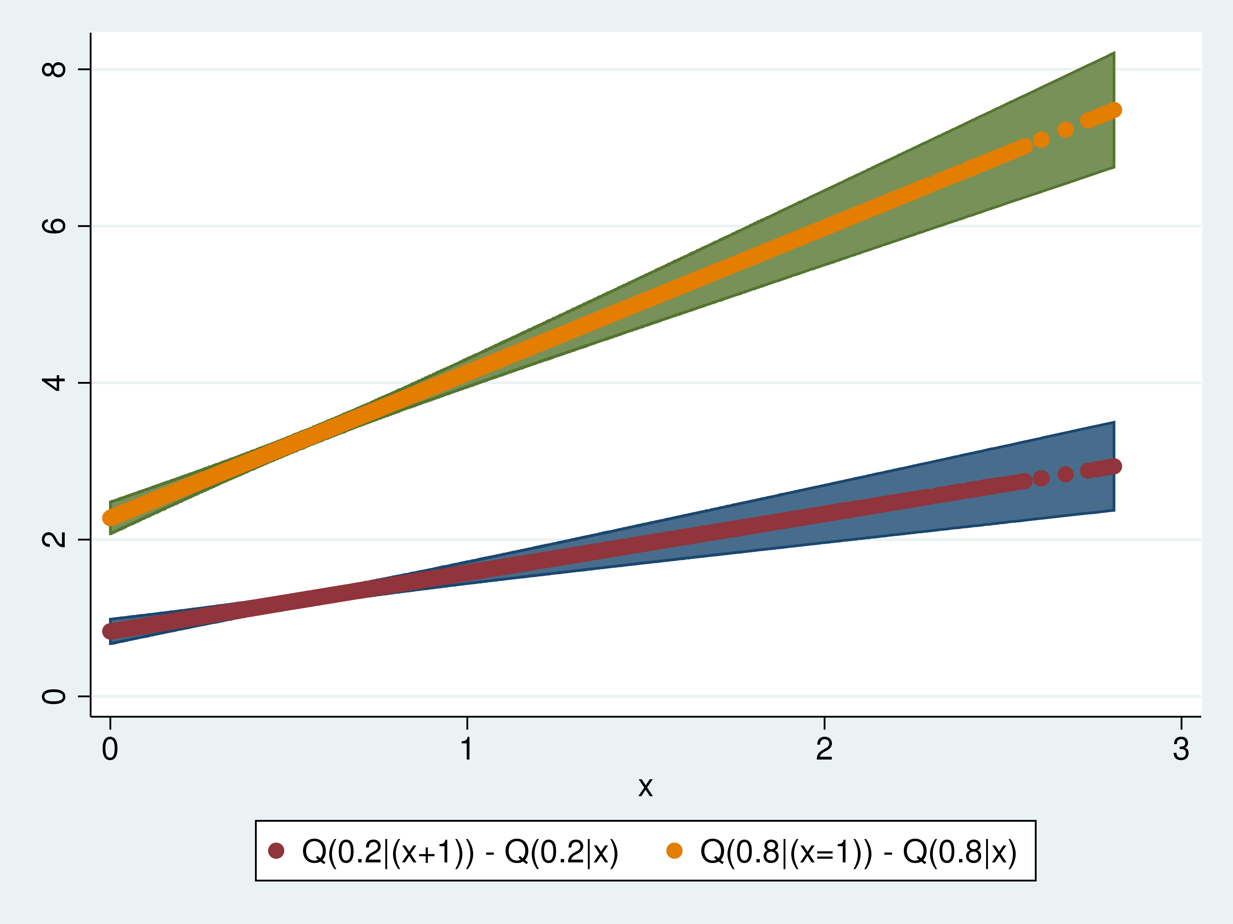
Both the magnitude and the slope of the effects are larger for the 0.8 conditional quantile function than for the 0.2 conditional quantile function.

Done and undone

I used simulated data to illustrate what conditional quantile functions are, and I illustrated that the effects of a covariate can vary over conditional quantiles.

References

Cameron, A. C., and P. K. Trivedi. 2010. Microeconometrics Using Stata. Rev. ed. College Station, TX: Stata Press.

Koenker, R., and G. Bassett. 1978. Regression quantiles. Econometrica 46: 33–50.

Wooldridge, J. M. 2010. Econometric Analysis of Cross Section and Panel Data. 2nd ed. Cambridge, MA: MIT Press.