Structural vector autoregression models
\(\def\bfy{{\bf y}}
\def\bfA{{\bf A}}
\def\bfB{{\bf B}}
\def\bfu{{\bf u}}
\def\bfI{{\bf I}}
\def\bfe{{\bf e}}
\def\bfC{{\bf C}}
\def\bfsig{{\boldsymbol \Sigma}}\)In my last post, I discusssed estimation of the vector autoregression (VAR) model,
\begin{align}
\bfy_t &= \bfA_1 \bfy_{t-1} + \dots + \bfA_k \bfy_{t-k} + \bfe_t \tag{1}
\label{var1} \\
E(\bfe_t \bfe_t’) &= \bfsig \label{var2}\tag{2}
\end{align}
where \(\bfy_t\) is a vector of \(n\) endogenous variables, \(\bfA_i\) are coefficient matrices, \(\bfe_t\) are error terms, and \(\bfsig\) is the covariance matrix of the errors.
In discussing impulse–response analysis last time, I briefly discussed the concept of orthogonalizing the shocks in a VAR—that is, decomposing the reduced-form errors in the VAR into mutually uncorrelated shocks. In this post, I will go into more detail on orthogonalization: what it is, why economists do it, and what sorts of questions we hope to answer with it.
Structural VAR
The simple VAR model in \eqref{var1} and \eqref{var2} provides a compact summary of the second-order moments of the data. If all we care about is characterizing the correlations in the data, then the VAR is all we need.
However, the reduced-form VAR may be unsatisfactory for two reasons, one relating to each equation in the VAR. First, \eqref{var1} allows for arbitrary lags but does not allow for contemporaneous relationships among its variables. Economic theory often links variables contemporaneously, and if we wish to use the VAR to test those theories, it must be modified to allow for contemporanous relationships among the model variables. A VAR that does allow for contemporanous relationships among its variables may be written as
\begin{align}
\bfA \bfy_t &= \bfC_1 \bfy_{t-1} + \dots + \bfC_k \bfy_{t-k} + \bfe_t
\label{var3}\tag{3}
\end{align}
and I need to introduce new notation (the \(\bfC_i\)) because when \(\bfA \neq \bfI\), the \(\bfC_i\) will generally differ from the \(\bfA_i\) in the reduced-form VAR. The \(\bfA\) matrix characterizes the contemporaneous relationships among the variables in the VAR.
The second deficiency of the reduced-form VAR is that its error terms will, in general, be correlated. We wish to decompose these error terms into mutually orthogonal shocks. Why is orthogonality so important? When we perform impulse–response analysis, we ask the question, “What is the effect of a shock to one equation, holding all other shocks constant?” To analyze that impulse, we need to keep other shocks fixed. But if the error terms are correlated, then a shock to one equation is associated with shocks to other equations; the thought experiment of holding all other shocks constant cannot be performed. The solution is to write the errors as a linear combination of “structural” shocks
\begin{align}
\bfe_t &= \bfB \bfu_t \label{var4}\tag{4}
\end{align}
Without loss of generality, we can impose \(E(\bfu_t\bfu_t’)=\bfI\).
So our task, then, is to estimate the parameters of a VAR that has been extended to include correlation among the endogenous variables and exclude correlation among the error terms. Combine \eqref{var3} and \eqref{var4} to obtain the structural VAR model,
\begin{align}
\bfA \bfy_t &= \bfC_1 \bfy_{t-1} + \dots + \bfC_k \bfy_{t-k}
+ \bfB \bfu_t \tag{5}
\end{align}
so the goal is to estimate \(\bfA\), \(\bfB\), and \(\bfC_i\). Unfortunately, there is little more we can say at this stage, because at this level of generality, the model’s parameters are not identified.
Identification
When the solutions to population-level moment equations are unique and produce the true parameters, the parameters are identified. In the VAR model, the population-level moment conditions use the second moments of the variables—variances, covariances, and autocovariances—as well as the covariance matrix of the error terms. The identification problem is to move from these moments back to unique estimates of the parameters in the structural matrices.
We can always estimate the reduced-form matrices \(\bfA_i\) and \(\bfsig\) from the VAR in \eqref{var1} and \eqref{var2}. We can then use the information in \((\bfA_i,\bfsig)\) to make inferences about \((\bfA,\bfB,\bfC_i)\). What does the structural VAR imply about the reduced-form moments? Assuming that \(\bfA\) is invertible, we can write the structural VAR as
\begin{align*}
\bfy_t &= \bfA^{-1} \bfC_1 \bfy_{t-1}
+ \dots
+ \bfA^{-1} \bfC_k \bfy_{t-k}
+ \bfA^{-1} \bfB \bfu_t
\end{align*}
which implies the following set of relationships,
\begin{align*}
\bfA^{-1}\bfC_i &= \bfA_i
\end{align*}
for \(i=1,2,\dots k\), and
\begin{align*}
\bfA^{-1} \bfB \bfB’ {\bfA^{-1}}’ &= \bfsig
\end{align*}
If we could form estimates of \(\bfA\) and \(\bfB\), then recovering the \(\bfC_i\) would be straightforward.
The problem is that there are many \(\bfA\) and \(\bfB\) matrices that are consistent with the same observed \(\bfsig\) matrix. Hence, without further information, we cannot uniquely pin down \(\bfA\) and \(\bfB\) from \(\bfsig\).
As a covariance matrix, \(\bfsig\) must be symmetric and hence has only \(n(n+1)/2\) pieces of information; however, \(\bfA\) and \(\bfB\) each have \(n^2\) parameters. We must place \(n^2+n(n-1)/2\) restrictions on \(\bfA\) and \(\bfB\) to obtain a unique estimate of \(\bfA\) and \(\bfB\) from \(\bfsig\). The order condition only ensures that we have enough restrictions. The rank condition ensures that we have enough linearly independent restrictions. It is most common to restrict some entries of \(\bfA\) or \(\bfB\) to zero or one.
Cholesky identification
The most common method of identification is to set \(\bfA=\bfI\) and to require \(\bfB\) to be a lower-triangular matrix, placing zeros on all entries above the diagonal. This identification scheme places \(n^2\) restrictions on \(\bfA\) and places \(n(n-1)/2\) restrictions on \(\bfB\), satisfying the order condition. The resulting mapping from structure to reduced form is
\begin{align}
\bfB \bfB’ = \bfsig \label{chol}
\tag{6}
\end{align}
along with the requirement that \(\bfB\) be lower triangular. There is a unique lower-triangular matrix \(\bfB\) that satisfies \eqref{chol}; hence, we can uniquely recover the structure from the reduced form. This identification scheme is often called “Cholesky” identification because the matrix \(\bfB\) can be recovered by taking a Cholesky decomposition of \(\bfsig\).
An equivalent method of identification is to let \(\bfA\) be lower triangular and let \(\bfB=\bfI\). Both of these methods may be thought of as imposing a causal ordering on the variables in the VAR: shocks to one equation contemporaneously affect variables below that equation but only affect variables above that equation with a lag. With this interpretation in mind, the causal ordering a researcher chooses reflects his or her beliefs about the relationships among variables in the VAR.
Suppose we have a VAR with three variables: inflation, the unemployment rate, and the interest rate. With the ordering (inflation, unemployment, interest rate), the shock to the inflation equation can affect all variables contemporaneously, but the shock to unemployment does not affect inflation contemporaneously, and the shock to the interest rate affects neither inflation nor unemployment contemporaneously. This ordering may reflect some beliefs the researcher has about the various shocks. For example, if one believes that monetary policy only affects other variables with a lag, it is appropriate to place monetary instruments like the interest rate last in the ordering. Different orderings reflect different assumptions about the underlying structure that the researcher is modeling.
With Cholesky identification, order matters: permuting the variables in the VAR will permute the entries in \(\bfsig\), which in turn will generate different \(\bfB\) matrices. The impulse responses one draws from the model are conditional on the ordering of the variables. One might be tempted, as a sort of robustness check, to try multiple orderings to see whether impulse responses varied much when the ordering changed. However, different orderings embed different assumptions about the relationships among variables, and it may or may not be sensible to think that an impulse response will be robust to those differing assumptions.
Example
Stata’s svar command estimates structural VARs. Let’s revisit the three-variable VAR from the previous post, this time using svar. The dataset can be accessed here. The following code block loads the data, sets up the \(\bfA\) and \(\bfB\) matrices, estimates the model, then creates impulse responses and stores them to a file.
. use usmacro.dta
. matrix A1 = (1,0,0 \ .,1,0 \ .,.,1)
. matrix B1 = (.,0,0 \ 0,.,0 \ 0,0,.)
. svar inflation unrate ffr, lags(1/6) aeq(A1) beq(B1)
Estimating short-run parameters
Iteration 0: log likelihood = -708.74354
Iteration 1: log likelihood = -443.10177
Iteration 2: log likelihood = -354.17943
Iteration 3: log likelihood = -303.90081
Iteration 4: log likelihood = -299.0338
Iteration 5: log likelihood = -298.87521
Iteration 6: log likelihood = -298.87514
Iteration 7: log likelihood = -298.87514
Structural vector autoregression
( 1) [a_1_1]_cons = 1
( 2) [a_1_2]_cons = 0
( 3) [a_1_3]_cons = 0
( 4) [a_2_2]_cons = 1
( 5) [a_2_3]_cons = 0
( 6) [a_3_3]_cons = 1
( 7) [b_1_2]_cons = 0
( 8) [b_1_3]_cons = 0
( 9) [b_2_1]_cons = 0
(10) [b_2_3]_cons = 0
(11) [b_3_1]_cons = 0
(12) [b_3_2]_cons = 0
Sample: 39 - 236 Number of obs = 198
Exactly identified model Log likelihood = -298.8751
------------------------------------------------------------------------------
| Coef. Std. Err. z P>|z| [95% Conf. Interval]
-------------+----------------------------------------------------------------
/a_1_1 | 1 (constrained)
/a_2_1 | .0348406 .0416245 0.84 0.403 -.046742 .1164232
/a_3_1 | -.3777114 .113989 -3.31 0.001 -.6011257 -.1542971
/a_1_2 | 0 (constrained)
/a_2_2 | 1 (constrained)
/a_3_2 | 1.402087 .1942736 7.22 0.000 1.021318 1.782857
/a_1_3 | 0 (constrained)
/a_2_3 | 0 (constrained)
/a_3_3 | 1 (constrained)
-------------+----------------------------------------------------------------
/b_1_1 | .4088627 .0205461 19.90 0.000 .3685931 .4491324
/b_2_1 | 0 (constrained)
/b_3_1 | 0 (constrained)
/b_1_2 | 0 (constrained)
/b_2_2 | .2394747 .0120341 19.90 0.000 .2158884 .263061
/b_3_2 | 0 (constrained)
/b_1_3 | 0 (constrained)
/b_2_3 | 0 (constrained)
/b_3_3 | .6546452 .0328972 19.90 0.000 .5901679 .7191224
------------------------------------------------------------------------------
. matlist e(A)
| inflation unrate ffr
-------------+---------------------------------
inflation | 1 0 0
unrate | .0348406 1 0
ffr | -.3777114 1.402087 1
. matlist e(B)
| inflation unrate ffr
-------------+---------------------------------
inflation | .4088627
unrate | 0 .2394747
ffr | 0 0 .6546452
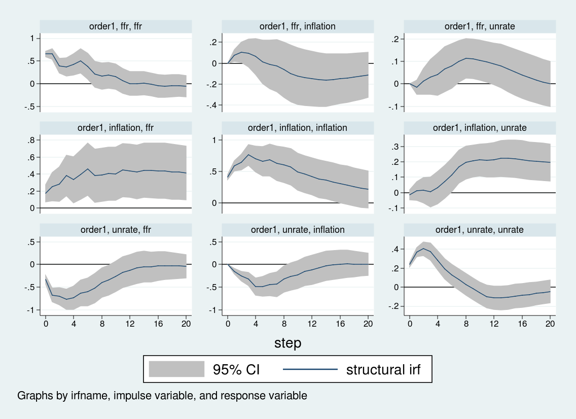
. irf create order1, set(var2.irf) replace step(20)
(file var2.irf created)
(file var2.irf now active)
irfname order1 not found in var2.irf
(file var2.irf updated)
. irf graph sirf, xlabel(0(4)20) irf(order1) yline(0,lcolor(black))
> byopts(yrescale)
The first two lines set up the \(\bfA\) and \(\bfB\) matrices. Missing values in those matrices indicate entries to be estimated; entries with given values are assumed to be fixed. I have restricted the diagonals of the \(\bfA\) matrix to unity, set elements above the main diagonal to zero, and allow the elements below the main diagonal to be estimated. Meanwhile, I allow the elements on the main diagonal of the \(\bfB\) matrix to be estimated but restrict the remaining entries to zero.
The third line runs the SVAR. The core of svar‘s syntax is familiar: we specify a list of variables and the lag length. The \(\bfA\) and \(\bfB\) matrices are passed to svar by the options aeq() and beq().
The output of svar focuses on the estimation of the \(\bfA\) and \(\bfB\) matrices; the estimated matrices on lagged endogenous variables are supressed by default. We can see that five of the six unrestricted entries are statistically significant; only the coefficient on inflation in the unemployment equation (/a_2_1) is statistically insignificant.
The matrices \(\bfA\) and \(\bfB\) may be of interest and can be accessed after estimation in e(A) and e(B). I display these matrices with matlist. You can get a sense for how the impulse responses will behave on impact by examining the \(\bfA\) matrix. By construction, inflation will not move on impact in response to the other two shocks. The unemployment rate will decline slightly on impact after an inflation shock, but we have already seen in the estimation output that this decline will be statistically insignificant. Meanwhile, the interest rate will rise in response to a rise in inflation but decline in response to a rise in the unemployment rate.
Finally, I create an irf file, var2.irf, and place the impulse responses into that file under the name order1.
Now, let’s estimate the structural VAR again but use a different ordering. We will place the interest rate first, then unemployment, then inflation. One way to accomplish that is to set the \(\bfA\) matrix to be upper triangular instead of lower triangular.
. matrix A2 = (1,.,. \ 0,1,. \ 0,0,1)

. matrix B2 = (.,0,0 \ 0,.,0 \ 0,0,.)

. svar inflation unrate ffr, lags(1/6) aeq(A2) beq(B2)
Estimating short-run parameters

Iteration 0:   log likelihood = -774.35412
Iteration 1:   log likelihood = -528.28591
Iteration 2:   log likelihood = -451.41967
Iteration 3:   log likelihood =  -358.6247
Iteration 4:   log likelihood = -302.25179
Iteration 5:   log likelihood = -298.92706
Iteration 6:   log likelihood = -298.87515
Iteration 7:   log likelihood = -298.87514

Structural vector autoregression

 ( 1)  [a_1_1]_cons = 1
 ( 2)  [a_2_1]_cons = 0
 ( 3)  [a_2_2]_cons = 1
 ( 4)  [a_3_1]_cons = 0
 ( 5)  [a_3_2]_cons = 0
 ( 6)  [a_3_3]_cons = 1
 ( 7)  [b_1_2]_cons = 0
 ( 8)  [b_1_3]_cons = 0
 ( 9)  [b_2_1]_cons = 0
 (10)  [b_2_3]_cons = 0
 (11)  [b_3_1]_cons = 0
 (12)  [b_3_2]_cons = 0

Sample:  39 - 236                               Number of obs     =        198
Exactly identified model                        Log likelihood    =  -298.8751

------------------------------------------------------------------------------
             |      Coef.   Std. Err.      z    P>|z|     [95% Conf. Interval]
-------------+----------------------------------------------------------------
      /a_1_1 |          1  (constrained)
      /a_2_1 |          0  (constrained)
      /a_3_1 |          0  (constrained)
      /a_1_2 |  -.0991471    .132311    -0.75   0.454     -.358472    .1601777
      /a_2_2 |          1  (constrained)
      /a_3_2 |          0  (constrained)
      /a_1_3 |  -.1391009   .0419791    -3.31   0.001    -.2213784   -.0568235
      /a_2_3 |   .1449874   .0200558     7.23   0.000     .1056788     .184296
      /a_3_3 |          1  (constrained)
-------------+----------------------------------------------------------------
      /b_1_1 |   .3972748   .0199638    19.90   0.000     .3581464    .4364031
      /b_2_1 |          0  (constrained)
      /b_3_1 |          0  (constrained)
      /b_1_2 |          0  (constrained)
      /b_2_2 |   .2133842    .010723    19.90   0.000     .1923676    .2344008
      /b_3_2 |          0  (constrained)
      /b_1_3 |          0  (constrained)
      /b_2_3 |          0  (constrained)
      /b_3_3 |   .7561185   .0379964    19.90   0.000     .6816469      .83059
------------------------------------------------------------------------------

. matlist e(A)

             | inflation     unrate        ffr
-------------+---------------------------------
   inflation |         1  -.0991471  -.1391009
      unrate |         0          1   .1449874
         ffr |         0          0          1

. matlist e(B)

             | inflation     unrate        ffr
-------------+---------------------------------
   inflation |  .3972748
      unrate |         0   .2133842
         ffr |         0          0   .7561185

. irf create order2, set(var2.irf) replace step(20)
(file var2.irf now active)
irfname order2 not found in var2.irf
(file var2.irf updated)

. irf graph sirf, xlabel(0(4)20) irf(order2) yline(0,lcolor(black))
> byopts(yrescale)
Again the first two lines set up the structural matrices, the third line estimates the VAR, the two matlist commands display the structural matrices, and I create and store the relevant impulse responses. Note that I give the impulse responses a name, order2, and store them in the same var2.irf file that holds the order1 impulse responses. Then, in the irf graph command, I use the irf() option to specify which set of impulse responses I wish to graph. In this way, you can store multiple impulse responses to the same file.
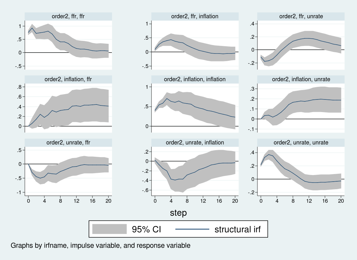
Although some of the impulse responses are similar, the response of inflation and unemployment to an interest rate shock differs sharply across the two orderings. When interest rates are ordered last, the inflation rate does not respond strongly to interest rate shocks, while the unemployment rate rises over about eight quarters before falling. By contrast, when the interest rate is ordered first, inflation actually rises on an interest rate shock, and the unemployment rate falls on impact before rising. The impulse response to an interest rate shock depends crucially on the Cholesky ordering.
Conclusion
In this post, I used svar to estimate a structural VAR and discussed some of the issues involved in estimating the parameters of structural VARs and interpreting their output. Using U.S. macroeconomic data, I showed one example where different identification assumptions produce markedly different inferences about the behavior of inflation and unemployment to an interest rate shock.