In Stata 14.2, we added the ability to use margins to estimate covariate effects after gmm. In this post, I illustrate how to use margins and marginsplot after gmm to estimate covariate effects for a probit model.

Margins are statistics calculated from predictions of a previously fit model at fixed values of some covariates and averaging or otherwise integrating over the remaining covariates. They can be used to estimate population average parameters like the marginal mean, average treatment effect, or the average effect of a covariate on the conditional mean. I will demonstrate how using margins is useful after estimating a model with the generalized method of moments.

Probit model

For binary outcome $y_i$ and regressors ${\bf x}_i$, the probit model assumes

$$\begin{equation} y_i = {\bf 1}({\bf x}_i{\boldsymbol \beta} + \epsilon_i > 0) \nonumber \end{equation}$$

where the error $\epsilon_i$ is standard normal. The indicator function ${\bf 1}(\cdot)$ outputs 1 when its input is true and outputs 0 otherwise.

The conditional mean of $y_i$ is

$$\begin{equation} E(y_i\vert{\bf x}_i) = \Phi({\bf x}_i{\boldsymbol \beta}) \nonumber \end{equation}$$

We can use the generalized method of moments (GMM) to estimate ${\boldsymbol \beta}$, with sample moment conditions

$$\begin{equation} \sum_{i=1}^N \left[\left\{ y_i \frac{\phi\left({\bf x}_i{\boldsymbol \beta}\right)}{\Phi\left({\bf x}_i{\boldsymbol \beta}\right)} – (1-y_i) \frac{\phi\left({\bf x}_i{\boldsymbol \beta}\right)}{\Phi\left(-{\bf x}_i{\boldsymbol \beta}\right)}\right\} {\bf x}_i\right] ={\bf 0} \nonumber \end{equation}$$

In addition to the model parameters ${\boldsymbol \beta}$, we may also be interested in the change in $y_i$ as we change one of the covariates in ${\bf x}_i$. How do individuals that only differ in the value of one of the regressors compare?

Suppose we want to compare differences in the regressor $x_{ij}$. The vector ${\bf x}_{i}^{\star}$ is ${\bf x}_{i}$ with the $j$th regressor $x_{ij}$ replaced by $x_{ij}+1$.

The effect of a unit change in $x_{ij}$ on $y_i$ at ${\bf x}_i$ is

$$\begin{eqnarray*} E(y_i\vert {\bf x}_i^{\star}) – E(y_i\vert {\bf x}_i) = \Phi\left({\bf x}_i^{\star}{\boldsymbol \beta}\right) – \Phi\left({\bf x}_i{\boldsymbol \beta}\right) \end{eqnarray*}$$

If we wanted to estimate how this effect changed over the population, we could add the following sample moment condition to our GMM estimation

$$\begin{equation} \sum_{i=1}^N \delta – \left[ \Phi\left({\bf x}_i^{\star}{\boldsymbol \beta}\right) – \Phi\left({\bf x}_i{\boldsymbol \beta}\right)\right] ={\bf 0} \nonumber \end{equation}$$

This condition implies

$$\begin{equation} \delta = \frac{1}{N}\sum_{i=1}^N \Phi\left({\bf x}_i^{\star}{\boldsymbol \beta}\right) – \Phi\left({\bf x}_i{\boldsymbol \beta}\right) ={\bf 0} \nonumber \end{equation}$$

Rather than using the condition for $\delta$ in the GMM estimation, we can directly calculate the sample average of the effect after estimation.

$$\begin{equation} \hat{\delta} = \frac{1}{N} \sum_{i=1}^N \Phi\left({\bf x}_i^{\star}\widehat{\boldsymbol \beta}\right) – \Phi\left({\bf x}_i\widehat{\boldsymbol \beta}\right) \nonumber \end{equation}$$

The standard error for this mean effect needs to be adjusted for the estimation of ${\boldsymbol \beta}$. We can use gmm to estimate ${\boldsymbol \beta}$ and then use margins to estimate $\delta$ and its properly adjusted standard error. This provides flexibility. You can estimate a model with few moment conditions and then estimate multiple margins.

Covariate effects

We estimate the mean effects for a probit regression model using gmm and margins from simulated data. We regress the binary $y_i$ on binary $d_i$ and continuous $x_i$ and $z_i$. A quadratic term for $x_i$ is included in the model, and we interact both powers of $x_i$ and $z_i$ with $d_i$.

First, we use gmm to estimate ${\boldsymbol \beta}$. Factor-variable notation is used to specify the quadratic power of $x_i$ and the interactions of the powers of $x_i$ and $z_i$ with $d_i$.

. gmm (cond(y,normalden({y: i.d##(c.x c.x#c.x c.z) i.d _cons})/   
>         normal({y:}),-normalden({y:})/normal(-{y:}))),  
>         instruments(i.d##(c.x c.x#c.x c.z) i.d) onestep

Step 1
Iteration 0:   GMM criterion Q(b) =  .26129294
Iteration 1:   GMM criterion Q(b) =  .01621062
Iteration 2:   GMM criterion Q(b) =  .00206357
Iteration 3:   GMM criterion Q(b) =  .00033537
Iteration 4:   GMM criterion Q(b) =  4.916e-06
Iteration 5:   GMM criterion Q(b) =  1.539e-08
Iteration 6:   GMM criterion Q(b) =  3.361e-13

note: model is exactly identified

GMM estimation

Number of parameters =   8
Number of moments    =   8
Initial weight matrix: Unadjusted                 Number of obs   =      5,000

------------------------------------------------------------------------------
             |               Robust
             |      Coef.   Std. Err.      z    P>|z|     [95% Conf. Interval]
-------------+----------------------------------------------------------------
         1.d |   1.752056   .0987097    17.75   0.000     1.558588    1.945523
           x |   .2209241   .0311227     7.10   0.000     .1599247    .2819235
             |
     c.x#c.x |  -.2864622   .0199842   -14.33   0.000    -.3256305   -.2472939
             |
           z |  -.6813765   .0558371   -12.20   0.000    -.7908152   -.5719379
             |
       d#c.x |
          1  |    .311213   .0543018     5.73   0.000     .2047835    .4176426
             |
   d#c.x#c.x |
          1  |  -.7297855   .0513903   -14.20   0.000    -.8305086   -.6290624
             |
       d#c.z |
          1  |  -.4272026   .0807842    -5.29   0.000    -.5855368   -.2688684
             |
       _cons |   .1180114   .0520303     2.27   0.023     .0160339    .2199888
------------------------------------------------------------------------------
Instruments for equation 1: 0b.d 1.d x c.x#c.x z 0b.d#co.x 1.d#c.x 0b.d#co.x#co.x 1.d#c.x#c.x 0b.d#co.z
    1.d#c.z _cons

Now, we use margins to estimate the mean effect of changing $x_i$ to $x_i+1$. We specify vce(unconditional) to estimate the mean effect over the population of $x_i$, $z_i$, and $d_i$. The normal probability expression is specified in the expression() option. The expression function xb() is used to get the linear prediction. We specify the at(generate()) option and atcontrast(r) under the contrast option so that the expression at $x_i$ will be subtracted from the expression at $x_i+1$. nowald is specified to suppress the Wald test of the contrast.

. margins, at(x=generate(x)) at(x=generate(x+1)) vce(unconditional) 
>         expression(normal(xb())) contrast(atcontrast(r) nowald)

Contrasts of predictive margins

Expression   : normal(xb())

1._at        : x               = x

2._at        : x               = x+1

--------------------------------------------------------------
             |            Unconditional
             |   Contrast   Std. Err.     [95% Conf. Interval]
-------------+------------------------------------------------
         _at |
   (2 vs 1)  |  -.0108121   .0040241     -.0186993    -.002925
--------------------------------------------------------------

Unit changes are particularly useful for evaluating the effect of discrete covariates. When a discrete covariate is specified using factor-variable notation, we can use contrast notation in margins to estimate the covariate effect.

We estimate the mean effect of changing from $d_i=0$ to $d_i=1$ over the population of covariates with margins. We specify the contrast r.d and the conditional mean in the expression() option. The expression will be evaluated at $d_i=0$ and then subtracted from the expression evaluated at $d_i=1$. We specify contrast(nowald) to suppress the Wald test of the contrast.

. margins r.d, expression(normal(xb())) vce(unconditional) contrast(nowald)

Contrasts of predictive margins

Expression   : normal(xb())

--------------------------------------------------------------
             |            Unconditional
             |   Contrast   Std. Err.     [95% Conf. Interval]
-------------+------------------------------------------------
           d |
   (1 vs 0)  |   .1370625   .0093206      .1187945    .1553305
--------------------------------------------------------------

So on average over the population, changing from $d_i=0$ to $d_i=1$ and keeping other covariates constant will increase the probability of success by 0.14.

Graphing covariate effects

We have used margins to estimate the mean covariate effect over the population of covariates. We can also use margins to estimate covariate effects at fixed values of the other covariates or to average the covariate effect over certain covariates while fixing others. We may examine multiple effects to find a pattern. The marginsplot command graphs effects estimated by margins and can be helpful in these situations.

Suppose we wanted to see how the effect of a unit change in $d_i$ varied over $x_i$. We can use margins with the at() option to estimate the effect at different values of $x_i$, averaged over the other covariates. We suppress the legend of fixed covariate values by specifying noatlegend.

. margins r.d, at(x = (-1 -.5 0 .5 1 1.5 2))      
>         expression(normal(xb())) noatlegend     
>         vce(unconditional) contrast(nowald)

Contrasts of predictive margins

Expression   : normal(xb())

--------------------------------------------------------------
             |            Unconditional
             |   Contrast   Std. Err.     [95% Conf. Interval]
-------------+------------------------------------------------
       d@_at |
 (1 vs 0) 1  |   .1536608   .0230032      .1085753    .1987462
 (1 vs 0) 2  |   .3446265   .0184594      .3084468    .3808062
 (1 vs 0) 3  |   .3907978    .017575      .3563515    .4252441
 (1 vs 0) 4  |   .3802466    .017735      .3454866    .4150066
 (1 vs 0) 5  |   .3166307   .0189175      .2795531    .3537083
 (1 vs 0) 6  |   .1182164   .0252829      .0686628      .16777
 (1 vs 0) 7  |  -.1053685   .0193225     -.1432399   -.0674971
--------------------------------------------------------------

The marginsplot command will graph these results for us.

. marginsplot

  Variables that uniquely identify margins: x

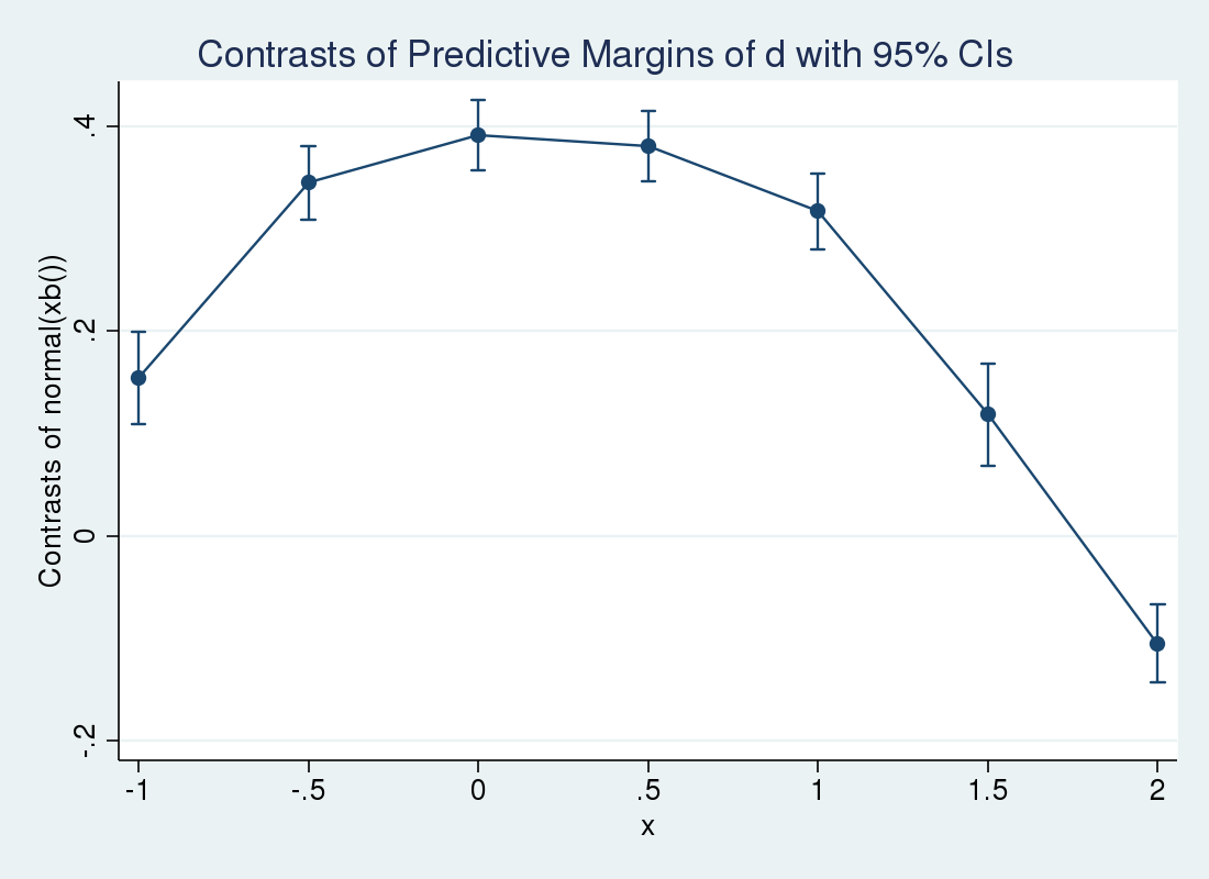
So the effect increases over small $x_i$ and decreases as $x_i$ grows large. We can use margins and marginsplot again to examine the conditional means at different values of $x_i$. This time, we specify the over() option so that separate predictions are made for $d_i=1$ and $d_i=0$. We expect to see the lines cross at a certain point, as the covariate effect crossed zero in the previous plot.

. margins, at(x = (-1 -.5 0 .5 1 1.5 2)) over(d)  
>         expression(normal(xb())) noatlegend     
>         vce(unconditional)

Predictive margins                              Number of obs     =      5,000

Expression   : normal(xb())
over         : d

------------------------------------------------------------------------------
             |            Unconditional
             |     Margin   Std. Err.      z    P>|z|     [95% Conf. Interval]
-------------+----------------------------------------------------------------
       _at#d |
        1 0  |   .2117609    .013226    16.01   0.000     .1858384    .2376834
        1 1  |   .3602933   .0194334    18.54   0.000     .3222046    .3983819
        2 0  |   .3042454   .0135516    22.45   0.000     .2776847    .3308061
        2 1  |   .6421908   .0142493    45.07   0.000     .6142627    .6701188
        3 0  |   .3616899   .0145202    24.91   0.000     .3332308     .390149
        3 1  |   .7455187   .0121556    61.33   0.000     .7216941    .7693432
        4 0  |      .3743    .014849    25.21   0.000     .3451965    .4034035
        4 1  |   .7475205   .0120208    62.19   0.000     .7239601    .7710809
        5 0  |   .3406649    .014334    23.77   0.000     .3125709     .368759
        5 1  |   .6504099   .0141534    45.95   0.000     .6226699      .67815
        6 0  |   .2651493   .0141303    18.76   0.000     .2374545    .2928442
        6 1  |   .3777989   .0215394    17.54   0.000     .3355825    .4200153
        7 0  |   .1642177    .014551    11.29   0.000     .1356982    .1927372
        7 1  |   .0565962   .0128524     4.40   0.000      .031406    .0817864
------------------------------------------------------------------------------

. marginsplot

  Variables that uniquely identify margins: x d

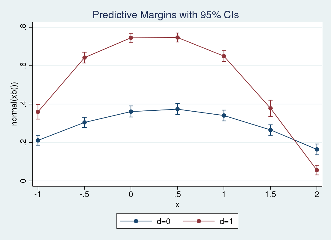
We see that the conditional means for $d_{i}=0$ rise above the means for $d_{i}=0$ at slightly below $x_i = 1.75$.

Differential effects

Instead of a unit change, we may be interested in the differential effect. This is the normalized effect on the mean of a small change in the covariate, the derivative of the mean with regard to the covariate $x_{ij}$. This is called the marginal or partial effect of $x_{ij}$ on $E(y_i\vert {\bf x}_i)$. See section 2.2.5 of Wooldridge (2010), section 5.2.4 of Cameron and Trivedi (2005), or section 10.6 of Cameron and Trivedi (2010) for more details. We can estimate the partial effect using margins, at fixed values of the regressors, or the mean partial effect over the population or sample.

We will use margins to estimate the mean marginal effects for the continuous covariates over the population of covariates. margins will take the derivatives for us if we specify dydx(). We only need to specify the form of the prediction. We again use the expression() option for this purpose.

. margins, expression(normal(xb())) vce(unconditional) dydx(x z)

Average marginal effects                        Number of obs     =      5,000

Expression   : normal(xb())
dy/dx w.r.t. : x z

------------------------------------------------------------------------------
             |            Unconditional
             |      dy/dx   Std. Err.      z    P>|z|     [95% Conf. Interval]
-------------+----------------------------------------------------------------
           x |   .0121859   .0045472     2.68   0.007     .0032736    .0210983
           z |  -.1439682   .0062519   -23.03   0.000    -.1562217   -.1317146
------------------------------------------------------------------------------

Conclusion

In this post, I have demonstrated how to use margins after gmm to estimate covariate effects for probit models. I also demonstrated how marginsplot can be used to graph covariate effects.

In future posts, we will use margins and marginsplot after gmm freely. This will let us perform marginal estimation and keep our moment conditions from becoming overcomplicated.

Appendix 1

The following code was used to generate the probit regression data.

. set seed 34

. quietly set obs 5000

. generate double x = 2*rnormal() + .1

. generate byte d = runiform() > .5

. generate double z = rchi2(1)

. generate double y = .2*x +.3*d*x - .3*(x^2) -.7*d*(x^2) 
>         -.8*z -.2*z*d + .2 + 1.5*d + rnormal() > 0

References

Cameron, A. C., and P. K. Trivedi. 2005. Microeconometrics: Methods and Applications. New York: Cambridge University Press.

——. 2010. Microeconometrics Using Stata. Rev. ed. College Station, TX: Stata Press.

Wooldridge, J. M. 2010. Econometric Analysis of Cross Section and Panel Data. 2nd ed. Cambridge, MA: MIT Press.