Introduction to Bayesian statistics, part 2: MCMC and the Metropolis–Hastings algorithm
In this blog post, I’d like to give you a relatively nontechnical introduction to Markov chain Monte Carlo, often shortened to “MCMC”. MCMC is frequently used for fitting Bayesian statistical models. There are different variations of MCMC, and I’m going to focus on the Metropolis–Hastings (M–H) algorithm. In the interest of brevity, I’m going to omit some details, and I strongly encourage you to read the [BAYES] manual before using MCMC in practice.
Let’s continue with the coin toss example from my previous post Introduction to Bayesian statistics, part 1: The basic concepts. We are interested in the posterior distribution of the parameter \(\theta\), which is the probability that a coin toss results in “heads”. Our prior distribution is a flat, uninformative beta distribution with parameters 1 and 1. And we will use a binomial likelihood function to quantify the data from our experiment, which resulted in 4 heads out of 10 tosses.
We can use MCMC with the M–H algorithm to generate a sample from the posterior distribution of \(\theta\). We can then use this sample to estimate things such as the mean of the posterior distribution.
There are three basic parts to this technique:
- Monte Carlo
- Markov chains
- M–H algorithm
Monte Carlo methods
The term “Monte Carlo” refers to methods that rely on the generation of pseudorandom numbers (I will simply call them random numbers). Figure 1 illustrates some features of a Monte Carlo experiment.
Figure 1: Proposal distributions, trace plots, and density plots
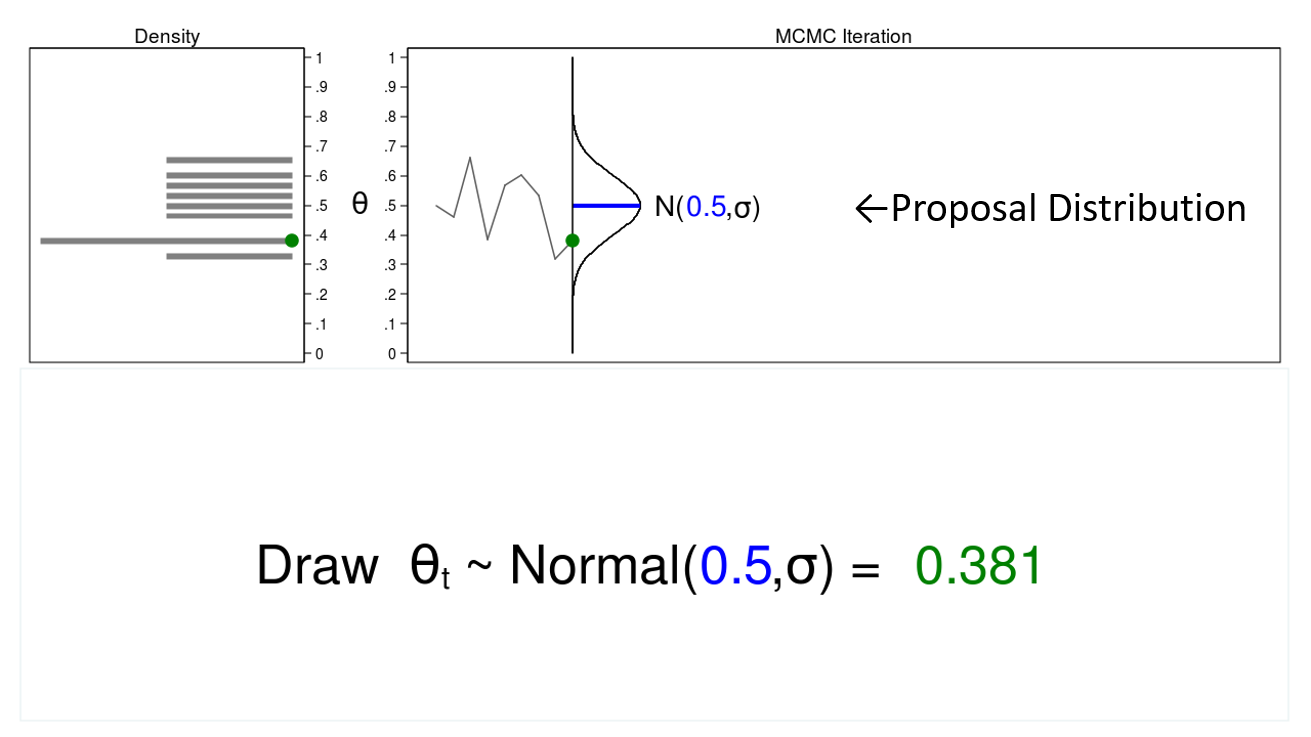
In this example, I will generate a series of random numbers from a normal distribution with a mean of 0.5 and some arbitrary variance, \(\sigma\). The normal distribution is called the proposal distribution.
The graph on the top right is called a trace plot, and it displays the values of \(\theta\) in the order in which they are drawn. It also displays the proposal distribution rotated clockwise 90 degrees, and I will shift it to the right each time I draw a value of theta. The green point in the trace plot shows the current value of \(\theta\).
The density plot on the top left is a histogram of the sample that is rotated counterclockwise 90 degrees. I have rotated the axes so that the \(\theta\) axes for both graphs are parallel. Again, the green point in the density plot shows the current value of \(\theta\).
Let’s draw 10,000 random values of \(\theta\) to see how this process works.
Animation 1: A Monte Carlo experiment
Animation 1 illustrates several important features. First, the proposal distribution does not change from one iteration to the next. Second, the density plot looks more and more like the proposal distribution as the sample size increases. And third, the trace plot is stationary—the pattern of variation looks the same over all iterations.
Our Monte Carlo simulation generated a sample that looks much like the proposal distribution, and sometimes that’s all we need. But we will require additional tools to generate a sample from our posterior distribution.
Markov chain Monte Carlo methods
A Markov chain is a sequence of numbers where each number is dependent on the previous number in the sequence. For example, we could draw values of \(\theta\) from a normal proposal distribution with a mean equal to the previous value of theta.
Figure 2 shows a trace plot and a density plot where the current value of \(\theta\) (\(\theta_t = 0.530\)) was drawn from a proposal distribution with a mean equal to the previous value of \(\theta\) (\(\theta_{t-1} = 0.712\)).
Figure 2: A draw from a MCMC experiment
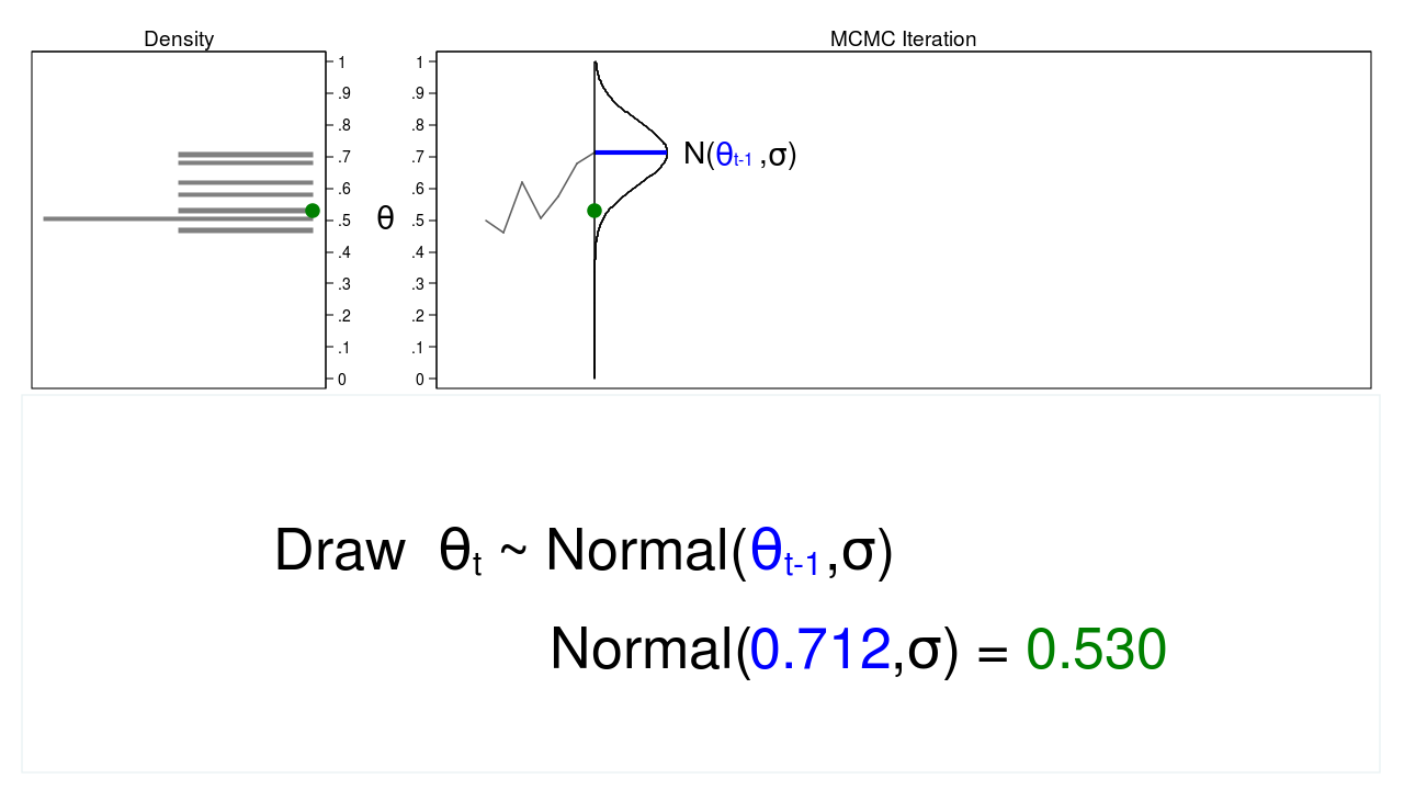
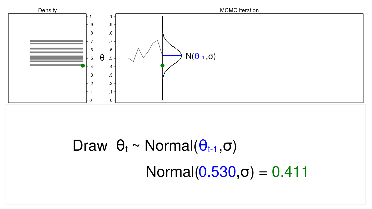
Figure 3 shows the trace plot and density plot for the next iteration in the sequence. The mean of the proposal density is now \(\theta_{t-1} = 0.530\), and we have drawn the random number (\(\theta_t = 0.411\)) from this new proposal distribution.
Figure 3: The next iteration of the MCMC experiment
Let’s draw 10,000 random values of \(\theta\) using MCMC to see how this process works.
Animation 2: A MCMC experiment
Animation 2 shows two differences between a Monte Carlo experiment and a MCMC experiment. First, the proposal distribution is changing with each iteration. This creates a trace plot with a “random walk” pattern: the variability is not the same over all iterations. Second, the resulting density plot does not look like the proposal distribution or any other useful distribution. It certainly doesn’t look like a posterior distribution.
The reason MCMC alone failed to generate a sample from the posterior distribution is that we haven’t incorporated any information about the
posterior distribution into the process of generating the sample. We could improve our sample by keeping proposed values of \(\theta\) that are more likely under the posterior distribution and discarding values that are less likely.
But the obvious difficulty with accepting and rejecting proposed values of \(\theta\) based on the posterior distribution is that we usually don’t know the functional form of the posterior distribution. If we knew the functional form, we could calculate probabilities directly without generating a random sample. So how can we accept or reject proposed values of \(\theta\) without knowing the functional form? One answer is the M–H algorithm!
MCMC and the M–H algorithm
The M–H algorithm can be used to decide which proposed values of \(\theta\) to accept or reject even when we don’t know the functional form of the posterior distribution. Let’s break the algorithm into steps and walk through several iterations to see how it works.
Figure 4: MCMC with the M–H algorithm: Iteration 1
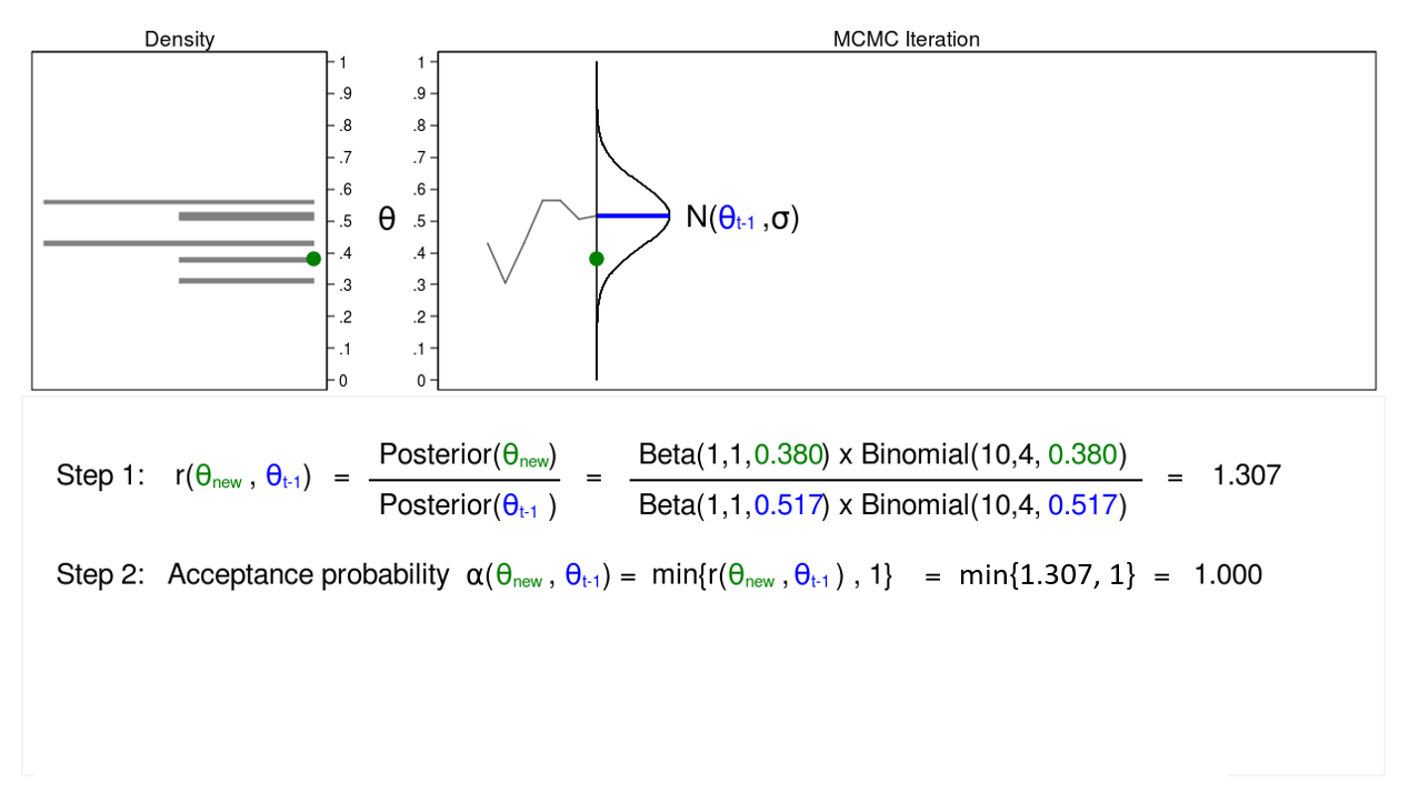
Figure 4 shows a trace plot and a density plot for a proposal distribution with mean equal to (\(\theta_{t-1} = 0.0.517\)). We have drawn a proposed value of \(\theta\), which is (\(\theta_\mathrm{new} = 0.380\)). I am referring to \(\theta_\mathrm{new}\) as “new” because I haven’t decided whether to accept or reject it yet.
We begin the M–H algorithm with step 1 by calculating the ratio
\[
r(\theta_\mathrm{new},\theta_{t-1}) = \frac{\mathrm{Posterior}(\theta_\mathrm{new})}{\mathrm{Posterior}(\theta_{t-1})}
\]
We don’t know the functional form of the posterior distribution, but in this example, we can substitute the product of the prior distribution and the likelihood function. The calculation of this ratio isn’t always this easy, but we’re trying to keep things simple.
Step 1 in figure 4 shows that the ratio of the posterior probabilities for (\(\theta_\mathrm{new} = 0.380\)) and (\(\theta_{t-1} = 0.0.517\)) equals 1.307. In step 2, we calculate the accept probability \(\alpha(\theta_\mathrm{new},\theta_{t-1})\), which is simply the minimum of the ratio \(r(\theta_\mathrm{new},\theta_{t-1})\) and 1. Step 2 is necessary because probabilities must fall between 0 and 1.
The acceptance probability equals 1, so we accept (\(\theta_\mathrm{new} = 0.380\)), and the mean of our proposal distribution becomes 0.380 in the next iteration.
Figure 5: MCMC with the M–H algorithm: Iteration 2
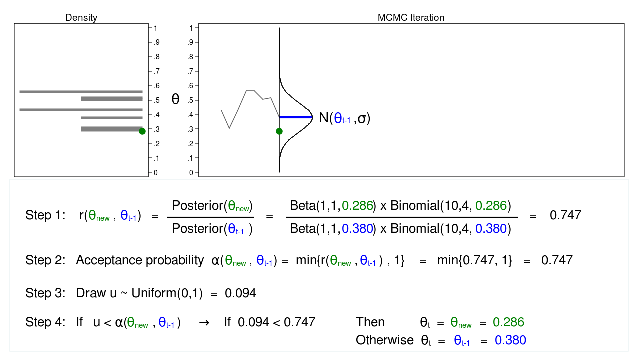
Figure 5 shows the next iteration where (\(\theta_\mathrm{new} = 0.286\)) has been drawn from our proposal distribution with mean (\(\theta_{t-1} = 0.380\)). The ratio, \(r(\theta_\mathrm{new},\theta_{t-1})\), calculated in step 1, equals 0.747, which is less than 1. The acceptance probability, \(\alpha(\theta_\mathrm{new},\theta_{t-1})\), calculated in step 2, equals 0.747.
We don’t automatically reject \(\theta_\mathrm{new}\) just because the acceptance probability is less than 1. Instead, we draw a random number, \(u\), from a \(\mathrm{Uniform}(0,1)\) distribution in step 3. If \(u\) is less than the acceptance probability, we accept the proposed value of \(\theta_\mathrm{new}\). Otherwise, we reject \(\theta_\mathrm{new}\) and keep \(\theta_{t-1}\).
Here \(u=0.094\) is less than the acceptance probability (0.747), so we will accept (\(\theta_\mathrm{new} = 0.286\)). I’ve displayed \(\theta_\mathrm{new}\) and 0.286 in green to indicate that they have been accepted.
Figure 6: MCMC with the M–H algorithm: Iteration 3
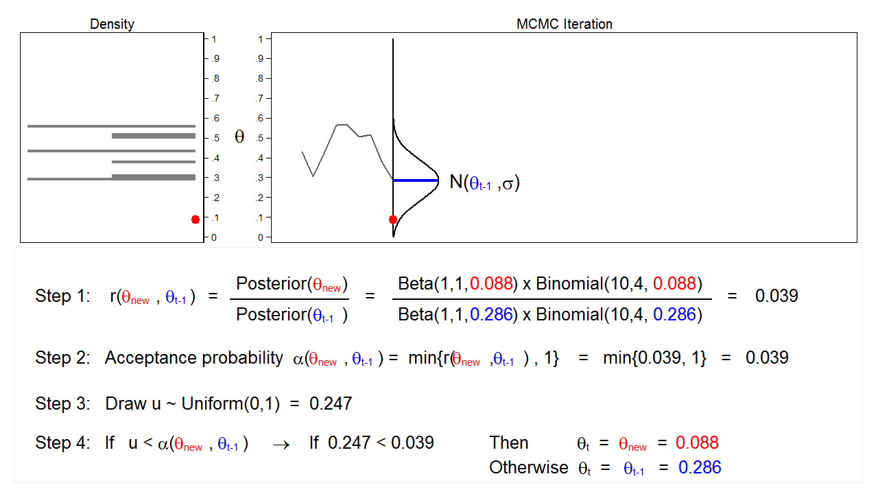
Figure 6 shows the next iteration where (\(\theta_\mathrm{new} = 0.088\)) has been drawn from our proposal distribution with mean (\(\theta_{t-1} = 0.286\)). The ratio, \(r(\theta_\mathrm{new},\theta_{t-1})\), calculated in step 1, equals 0.039, which is less than 1. The acceptance probability, \(\alpha(\theta_\mathrm{new},\theta_{t-1})\), calculated in step 2, equals 0.039. The value of \(u\), calculated in step 3, is 0.247, which is greater than the acceptance probability. So we reject \(\theta_\mathrm{new}=0.088\) and keep \(\theta_{t-1} = 0.286\) in step 4.
Let’s draw 10,000 random values of \(\theta\) using MCMC with the M–H algorithm to see how this process works.
Animation 3: MCMC with the M–H algorithm
Animation 3 illustrates several things. First, the proposal distribution changes with most iterations. Note that proposed values of \(\theta_\mathrm{new}\) are displayed in green if they are accepted and red if they are rejected. Second, the trace plot does not exhibit the random walk pattern we observed using MCMC alone. The variation is similar across all iterations, And third, the density plot looks like a useful distribution.
Let’s rotate the resulting density plot and take a closer look.
Figure 7: A sample from the posterior distribution generated with MCMC with the M–H algorithm
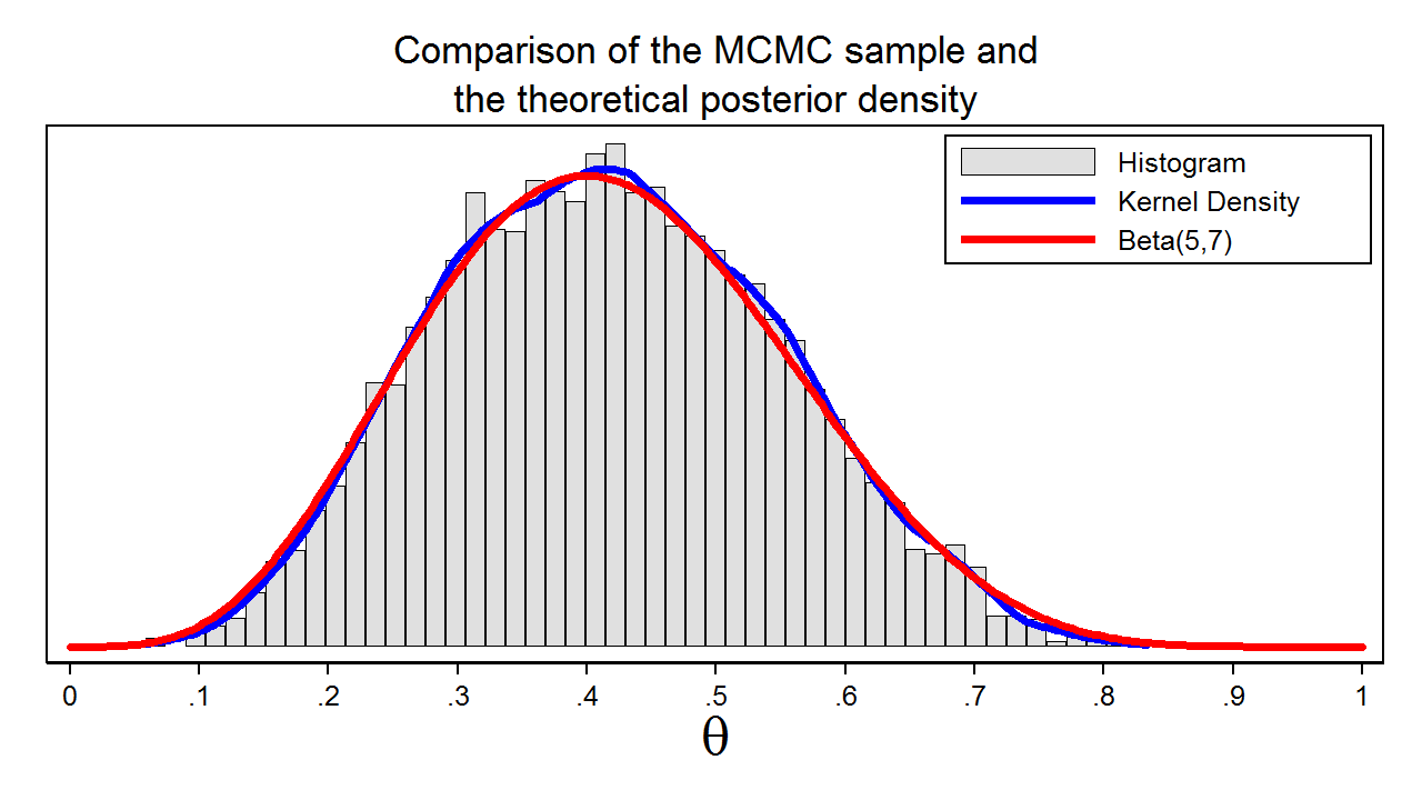
Figure 7 shows a histogram of the sample that we generated using MCMC with the M–H algorithm. In this example, we know that the posterior distribution is a beta distribution with parameters 5 and 7. The red line shows the analytical posterior distribution, and the blue line is a kernel density plot for our sample. The kernel density plot is quite similar to the Beta(5,7) distribution, which suggests that our sample is a good approximation to the theoretical posterior distribution.
We could then use our sample to calculate the mean or median of the posterior distribution, a 95% credible interval, or the probability that \(\theta\) falls within an arbitrary interval.
MCMC and the M–H algorithm in Stata
Let’s return to our coin toss example using bayesmh.
We specified a beta distribution with parameters 1 and 1 along with a binomial likelihood.
Example 1: Using bayesmh with a Beta(1,1) prior
. bayesmh heads, likelihood(dbernoulli({theta})) prior({theta}, beta(1,1))

Burn-in ...
Simulation ...

Model summary
------------------------------------------------------------------------------
Likelihood:
  heads ~ bernoulli({theta})

Prior:
  {theta} ~ beta(1,1)
------------------------------------------------------------------------------

Bayesian Bernoulli model                         MCMC iterations  =     12,500
Random-walk Metropolis-Hastings sampling         Burn-in          =      2,500
                                                 MCMC sample size =     10,000
                                                 Number of obs    =         10
                                                 Acceptance rate  =      .4454
Log marginal likelihood = -7.7989401             Efficiency       =      .2391

------------------------------------------------------------------------------
             |                                                Equal-tailed
             |      Mean   Std. Dev.     MCSE     Median  [95% Cred. Interval]
-------------+----------------------------------------------------------------
       theta |  .4132299   .1370017   .002802   .4101121    .159595   .6818718
------------------------------------------------------------------------------
The output header tells us that bayesmh ran 12,500 MCMC iterations. “Burn-in” tells us that 2,500 of those iterations were discarded to reduce the influence of the random starting value of the chain. The next line in the output tells us that the final MCMC sample size is 10,000, and the next line tells us that there were 10 observations in our dataset. The acceptance rate is the proportion of proposed values of \(\theta\) that were included in our final MCMC sample. I’ll refer you to the Stata Bayesian Analysis Reference Manual for a definition of efficiency, but high efficiency indicates low autocorrelation, and low efficiency indicates high autocorrelation. The Monte Carlo standard error (MCSE), shown in the coefficient table, is an approximation of the error in estimating the true posterior mean.
Checking convergence of the chain
The term “convergence” has a different meaning in the context of MCMC than in the context of maximum likelihood. Algorithms used for maximum likelihood estimation iterate until they converge to a maximum. MCMC chains do not iterate until an optimum value is identified. The chain simply iterates until the desired sample size is reached, and then the algorithm stops. The fact that the chain stops running does not indicate that an optimal sample from the posterior distribution has been generated. We must examine the sample to check for problems. We can examine the sample graphically using bayesgraph diagnostics.
. bayesgraph diagnostics {theta}
Figure 8: Diagnostic plots
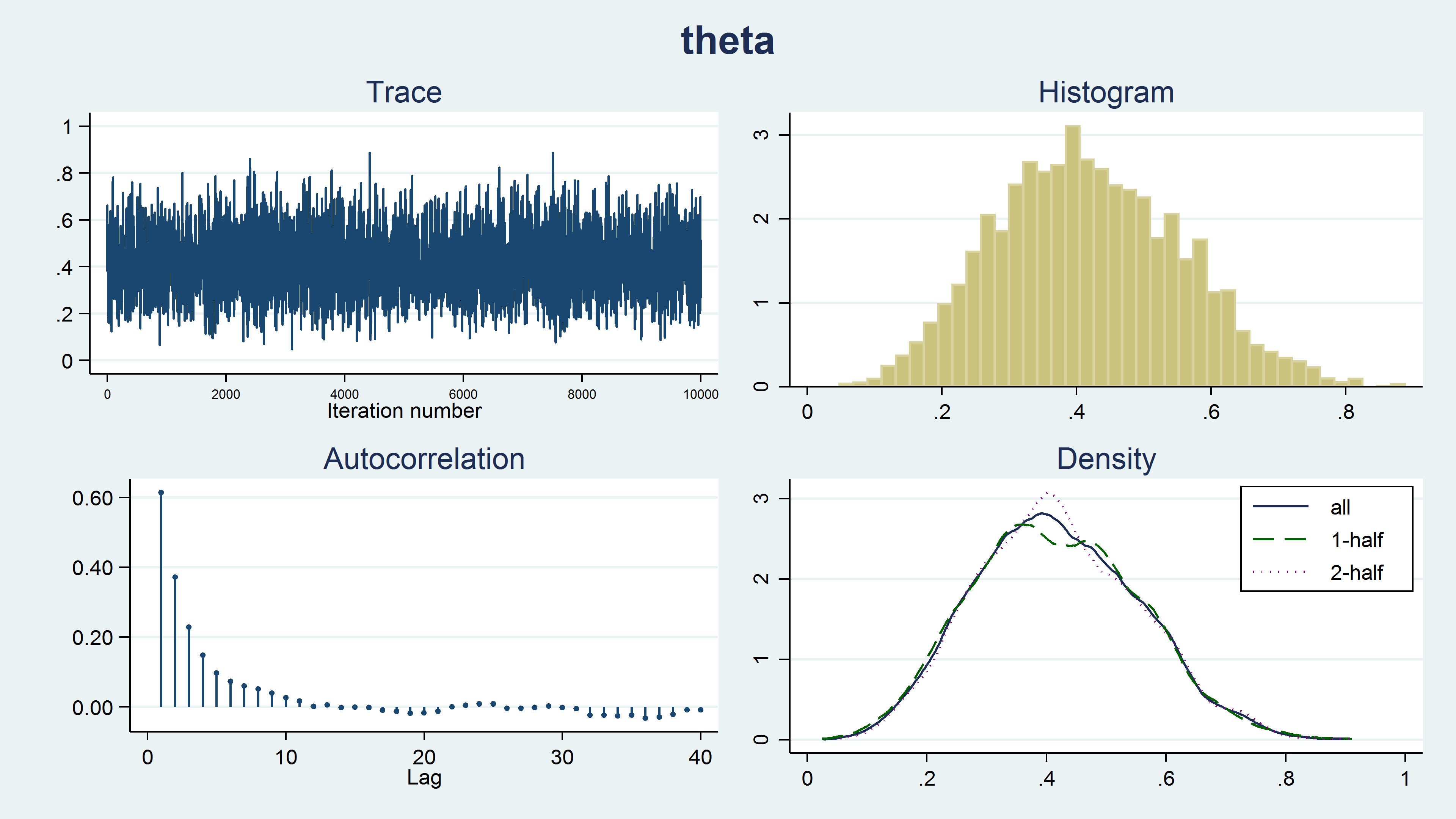
Figure 8 shows a diagnostic graph that contains a trace plot, a histogram and density plots for our MCMC sample, and a correlegram. The trace plot has a stationary pattern, which is what we would like to see. The random walk pattern shown in animation 2 indicates problems with the chain. The histogram doesn’t have any unusual features such as multiple modes. The kernel density plots for the full sample, the first half of the chain, and the last half of the chain all look similar and don’t show any strange features such as different densities for the first and last half of the chain. Generating the sample using a Markov chain leads to autocorrelation in the sample, but the autocorrelation decreases quickly for larger lag values. None of these plots indicate any problems with our sample.
Summary
This blog post introduced the idea behind MCMC using the M–H algorithm. Note that I have omitted some details and ignored some assumptions so that we could keep things simple and develop our intuition. Stata’s bayesmh command actually implements a much more sophisticated algorithm called adaptive MCMC with the M–H algorithm. But the basic idea is the same, and I hope I’ve inspired you to try it out.
You can view a video of this topic on the Stata Youtube Channel here:
Introduction to Bayesian Statistics, part 2: MCMC and the Metropolis Hastings algorithm