In this blog post, I’d like to give you a relatively nontechnical introduction to Bayesian statistics. The Bayesian approach to statistics has become increasingly popular, and you can fit Bayesian models using the bayesmh command in Stata. This blog entry will provide a brief introduction to the concepts and jargon of Bayesian statistics and the bayesmh syntax. In my next post, I will introduce the basics of Markov chain Monte Carlo (MCMC) using the Metropolis–Hastings algorithm.

Bayesian statistics by example

Many of us were trained using a frequentist approach to statistics where parameters are treated as fixed but unknown quantities. We can estimate these parameters using samples from a population, but different samples give us different estimates. The distribution of these different estimates is called the sampling distribution, and it quantifies the uncertainty of our estimate. But the parameter itself is still considered fixed.

The Bayesian approach is a different way of thinking about statistics. Parameters are treated as random variables that can be described with probability distributions. We don’t even need data to describe the distribution of a parameter—probability is simply our degree of belief.

Let’s work through a coin toss example to develop our intuition. I will refer to the two sides of the coin as “heads” and “tails”. If I toss the coin in the air, it must land on either the “heads” side or the “tails” side, and I will use \(\theta\) to denote the probability that the coin lands with the “heads” side facing up.

Prior distributions

The first step in our Bayesian example is to define a prior distribution for \(\theta\). A prior distribution is a mathematical expression of our belief about the distribution of the parameter. The prior distribution can be based on our experience or assumptions about the parameter, or it could be a simple guess. For example, I could use a uniform distribution to express my belief that the probability of “heads” could be anywhere between zero and one with equal probability. Figure 1 shows a beta distribution with parameters one and one that is equivalent to a uniform distribution on the interval zero to one.

Figure 1: Uninformative Beta(1,1) Prior

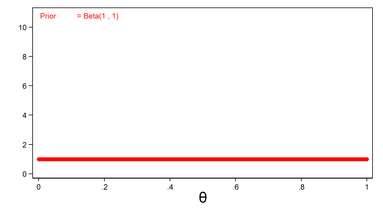
My beta(1,1) distribution is called an uninformative prior because all values of the parameter have equal probability.

Common sense would suggest that the probability of heads is closer to 0.5, and I could express this belief mathematically by increasing the parameters of my beta distribution. Figure 2 shows a beta distribution with parameters 30 and 30.

Figure 2: Informative Beta(30,30) Prior

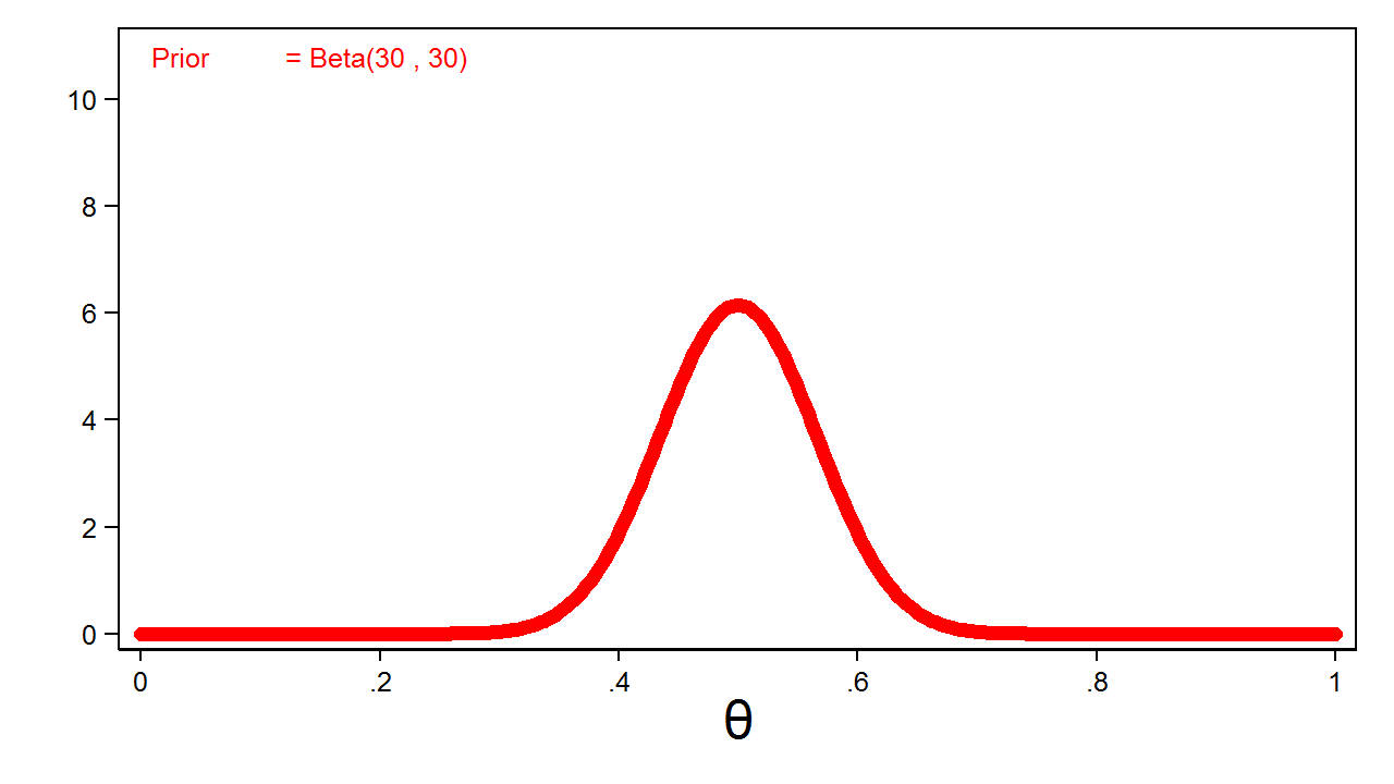
Figure 2 is called an informative prior because all values of the parameter do not have equal probability.

Likelihood functions

The second step in our Bayesian example is to collect data and define a likelihood function. Let’s say that I toss the coin 10 times and observe 4 heads. I then enter my results in Stata so that I can use the data later.

clear
input heads
0
0
1
0
0
1
1
0
0
1
end

Next, I need to specify a likelihood function for my data. Probability distributions quantify the probability of the data for a given parameter value (that is, \(P(y|\theta)\)), whereas a likelihood function quantifies the likelihood of a parameter value given the data (that is, \(L(\theta|y)\)). The functional form is the same for both, and the notation is often used interchangeably (that is, \(P(y|\theta) = L(\theta|y)\)).

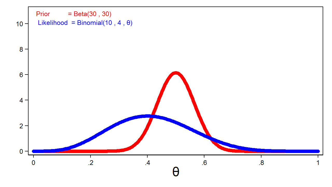
The binomial probability distribution is often used to quantify the probability of the number of successes out of a fixed number of trials. Here I can quantify the results of my experiment using a binomial likelihood function that quantifies the likelihood of \(\theta\) given 4 heads out of 10 tosses.

The blue line in figure 4 shows a binomial likelihood function for theta given 4 heads out of 10 coin tosses. I have rescaled the graph of the likelihood function so that the area under the curve equals one. This allows me to compare the likelihood function with the prior distribution graphed in red.

Figure 3: The Binomial(4,10,\(\boldsymbol{\theta}\)) Likelihood Function and the Beta(30,30) Prior Distribution

Posterior distributions

The third step in our Bayesian example is to calculate a posterior distribution. This allows us to update our belief about the parameter with the results of our experiment. In simple cases, we can compute a posterior distribution by multiplying the prior distribution and the likelihood function. Technically, the posterior is proportional to the product of the prior and the likelihood, but let’s keep things simple for now.

\[\mathrm{Posterior} = \mathrm{Prior}*\mathrm{Likelihood}\]
\[P(\theta|y) = P(\theta)*P(y|\theta)\]
\[P(\theta|y) = \mathrm{Beta}(\alpha,\beta)*\mathrm{Binomial}(n,y,\theta)\]
\[P(\theta|y) = \mathrm{Beta}(y+\alpha,n-y+\beta)\]

In this example, the beta distribution is called a “conjugate prior” for the binomial likelihood function because the posterior distribution belongs to the same distribution family as the prior distribution. Both the prior and the posterior have beta distributions.

Figure 4 shows the posterior distribution of theta with the prior distribution and the likelihood function.

Figure 4: The Posterior Distribution, the Likelihood Function, and the Prior Distribution

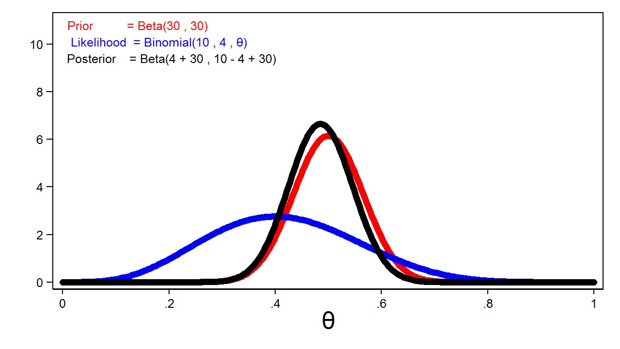
Notice that the posterior closely resembles the prior distribution. This is because we used an informative prior and a relatively small sample size.

Let’s explore the effect of different priors and sample sizes on the posterior distribution. The red line in figure 5 shows a completely uninformative \(\mathrm{Beta}(1,1)\) prior, and the likelihood function is plotted in blue. You can’t see the blue line because it is masked by the posterior distribution, which is plotted in black.

Figure 5: The Posterior Distribution For a Beta(1,1) Prior Distribution

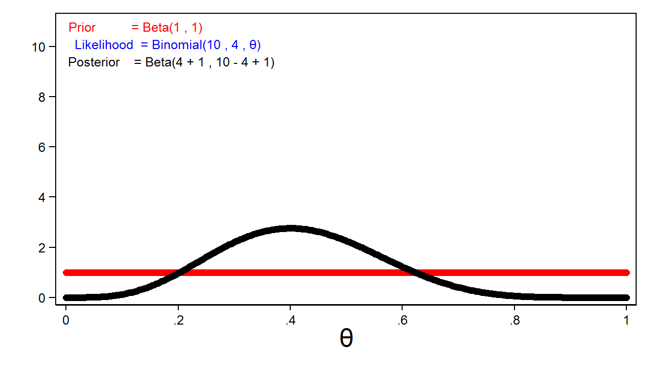
This is an important feature of Bayesian analysis: the posterior distribution will usually be equivalent to the likelihood function when we use completely uninformative priors.

Animation 1 shows that more informative priors will have greater influence on the posterior distribution for a given sample size.

Animation 1: The effect of more informative prior distributions on the posterior distribution

Animation 2 shows that larger sample sizes will give the likelihood function more influence on the posterior distribution for a given prior distribution.

Animation 2: The effect of larger sample sizes on the posterior distribution

In practice, this means that we can reduce the standard deviation of the posterior distribution using smaller sample sizes when we use more informative priors. But a similar reduction in the standard deviation may require a larger sample size when we use a weak or uninformative prior.

After we calculate the posterior distribution, we can calculate the mean or median of the posterior distribution, a 95% equal tail credible interval, the probability that theta lies within an interval, and many other statistics.

Example using bayesmh

Let’s analyze our coin toss experiment using Stata’s bayesmh command. Recall that I saved our data in the variable heads above. In the bayesmh command in Example 1, I will denote our parameter {theta}, specify a Bernoulli likelihood function, and use an uninformative beta(1,1) prior distribution.

Example 1: Using bayesmh with a Beta(1,1) prior

. bayesmh heads, likelihood(dbernoulli({theta})) prior({theta}, beta(1,1))       

Burn-in ...
Simulation ...

Model summary
------------------------------------------------------------------------------
Likelihood:
  heads ~ bernoulli({theta})

Prior:
  {theta} ~ beta(1,1)
------------------------------------------------------------------------------

Bayesian Bernoulli model                         MCMC iterations  =     12,500
Random-walk Metropolis-Hastings sampling         Burn-in          =      2,500
                                                 MCMC sample size =     10,000
                                                 Number of obs    =         10
                                                 Acceptance rate  =      .4454
Log marginal likelihood = -7.7989401             Efficiency       =      .2391

------------------------------------------------------------------------------
             |                                                Equal-tailed
             |      Mean   Std. Dev.     MCSE     Median  [95% Cred. Interval]
-------------+----------------------------------------------------------------
       theta |  .4132299   .1370017   .002802   .4101121    .159595   .6818718
------------------------------------------------------------------------------

Let’s focus on the table of coefficients and ignore the rest of the output for now. We’ll discuss MCMC next week. The output tells us that the mean of our posterior distribution is 0.41 and that the median is also 0.41. The standard deviation of the posterior distribution is 0.14, and the 95% credible interval is [\(0.16 – 0.68\)]. We can interpret the credible interval the way we would often like to interpret confidence intervals: there is a 95% chance that theta falls within the credible interval.

We can also calculate the probability that theta lies within an arbitrary interval. For example, we could use bayestest interval to calculate the probability that theta lies between 0.4 and 0.6.

Example 2: Using bayestest interval to calculate probabilities

. bayestest interval {theta}, lower(0.4) upper(0.6)

Interval tests     MCMC sample size =    10,000

       prob1 : 0.4 < {theta} < 0.6

-----------------------------------------------
             |      Mean    Std. Dev.      MCSE
-------------+---------------------------------
       prob1 |     .4265     0.49459   .0094961
-----------------------------------------------

Our results show that there is a 43% chance that theta lies between 0.4 and 0.6.

Why use Bayesian statistics?

There are many appealing features of the Bayesian approach to statistics. Perhaps the most appealing feature is that the posterior distribution from a previous study can often serve as the prior distribution for subsequent studies. For example, we might conduct a small pilot study using an uninformative prior distribution and use the posterior distribution from the pilot study as the prior distribution for the main study. This approach would increase the precision of the main study.

Summary
In this post, we focused on the concepts and jargon of Bayesian statistics and worked a simple example using Stata's bayesmh command. Next time, we will explore MCMC using the Metropolis–Hastings algorithm.

You can view a video of this topic on the Stata Youtube Channel here:

Introduction to Bayesian Statistics, part 1: The basic concepts