We announced Stata 15 today. It’s a big deal because this is Stata’s biggest release ever.

I posted to Statalist this morning and listed sixteen of the most important new features. Here on the blog I will say more about them, and you can learn even more by visiting our website and seeing the Stata 15 features page.

I go into depth below on the sixteen highlighted features. They are (click to jump)

 

1. Extended regression models
2. Latent class analysis (LCA)
3. Bayesian prefix command
4. Linearized dynamic stochastic general equilibrium (DSGE) models
5. Dynamic Markdown documents for the web
6. Nonlinear mixed-effects models
7. Spatial autoregressive models (SAR)
8. Interval-censored parametric survival-time models
9. Finite mixture models (FMMs)
10. Mixed logit models
11. Nonparametric regression
12. Power analysis for cluster randomized designs and regression models
13. Word and PDF documents
14. Graph color transparency/opacity
15. ICD-10-CM/PCS support
16. Federal Reserve Economic Data (FRED) support
17. And more

The sixteen features listed above certainly important ones, but there are others worthy of mention. More come readily to mind:

• Bayesian multilevel models
• Threshold regression
• Panel-data tobit with random coefficients
• Multilevel regression for interval-measured outcomes
• Multilevel tobit regression for censored outcomes
• Panel data cointegration tests
• Tests for multiple breaks in time series
• Multiple-group generalized SEM
• Heteroskedastic linear regression
• Poisson models with Heckman-style sample selection
• Panel-data nonlinear models with random coefficients
• Bayesian panel-data models
• Panel-data interval regression with random coefficients
• SVG export
• Bayesian survival models
• Zero-inflated ordered probit
• Add your own power and sample-size methods
• Bayesian sample-selection models
• Stata in Swedish
• Improvements to the Do-file Editor
• Stream random-number generator
• Improvements for Java plugins
• More parallelization in Stata/MP

 

1. Extended regression models

We call them ERMs—extended regression models. Four new commands fit

• linear regressions,
• interval regressions including tobit,
• probit, and
• ordered probit models

with any combination of

• endogenous covariates,
• nonrandom treatment assignment, and
• endogenous (Heckman-style) sample selection.

These new commands are just short of amazing because you can put endogenous covariates in any of the equations, and that includes the treatment-assignment and probit-selection equations. And endogenous covariates are not limited to being continuous. They can be binary or ordinal. And they can be interacted with other covariates, whether exogenous or endogenous. They can even be interacted with themselves to form squared or cubic terms!

These new ERM commands—eregress, eintreg, eprobit, and eoprobit—are destined to become popular because they address so many of the problems researchers have. First, you might have an endogenous variable because lots of models have omitted variables that are correlated with the variables in the model. Next, data are often censored, and the censoring is not random. ERM sample-selection options allow you to model the sample-selection process and so adjust for it. Or if you are fitting a treatment-effects model with nonrandom assignment, you can use ERM treatment-assignment options. Or you can combine the treatment-assignment and selection options, which will be of special interest to those fitting endogenous treatment-assignment models in which some are lost because of follow-up.

The syntax is simple:

. eregress   y x1 x2

. eregress   y x1 x2,  endogenous(       x2 = x3 x4, nomain)

. eregress   y x1 x2,  endogenous(       x2 = x3 x4, nomain) 
                           select( selected = x2 x5)          

. eregress   y x1 x2,  endogenous(       x2 = x3 x4, nomain) 
                          entreat(  treated = x2 x5)          

. eregress   y x1 x2,  endogenous(      x2 = x3 x5, nomain)
                          entreat( treated = x2 x3 x4)          
                           select(selected = x2 x6)          

eregress fits linear regressions. You can just as easily fit a probit model as a linear regression model. If the outcome variable y is binary, type

. eprobit    y x1 x2,  endogenous(      x2 = x3 x5, nomain)
                          entreat( treated = x2 x3 x4)
                           select(selected = x2 x6) 

If the outcome variable y is continuous but the variable x2 is binary, type

. eregress   y x1 x2,  endogenous(     x2 = x3 x5, binary nomain)
                         entreat( treated = x2 x3 x4) 
                          select(selected = x2 x6)  

If both y and x2 are binary, type

. eprobit    y x1 x2,  endogenous(     x2 = x3 x5, binary nomain)
                         entreat( treated = x2 x3 x4) 
                          select(selected = x2 x6)  

In case you are wondering about the strange nomain option, it is a detail. When you specify endogenous(name=…), variable name is added to the main equation automatically. You can type

. eregress y x1,     endogenous(x2=x3 x4)

or

. eregress y x1 x2,  endogenous(x2=x3 x4, nomain)

and, either way, the same model is fit. I specified nomain in the opening examples just so I would not have to explain that the option included x2 in the main equation.

See the examples at the Stata 15 ERMs page.

Back to highlights.

 

2. Latent class analysis (LCA)

Latent means unobserved. Class means group. Latent classes are unobserved groups within your data. You might have data on consumers and believe they are divided into three groups depending on their potential interest in your product. Unfortunately, you do not have variables in the data specifying the group to which each consumer belongs. If you have four binary variables that are indicators of the latent class to which consumers belong, however, you can type

. gsem (y1 y2 y3 y4 <- cons), lclass(Consum 3) logit

y1, y2, y3, and y4 are observed. Consum is the latent categorical variable that lclass(Consum 3) specified as taking on three values. The result is to fit a model in which y1, y2, y3, and y4 are determined by unobserved class.

The command fits 4x3=12 logistic regressions, one for each of the four y variables and each of the three classes. Each regression has an intercept. In addition, a multinomial logistic regression is also fit to predict Consum.

After fitting the model, you can

• use the new estat lcprob command to estimate the proportion of consumers belonging to each class;
• use the new estat lcmean command to estimate the marginal means of y1, y2, y3, and y4 in each class (the means will be probabilities for the example shown);
• use the new estat lcgof command to evaluate the goodness of fit; and
• use the existing predict command to obtain predicted probabilities of class membership and predicted values of observed outcome variables.

See more at the Stata 15 Latent class analysis page.

Back to highlights.

 

3. Bayesian prefix command

The new bayes: prefix command lets you fit a wider range of Bayesian models than were previously available. You always could fit a Bayesian linear regression, but now you can fit it by typing

. bayes: regress y x1 x2 

That is convenient. What you could not previously do was fit a Bayesian survival model. Now you can:

. bayes: streg x1 x2, distribution(weibull) 

You can even fit Bayesian multilevel survival models:

. bayes: streg x1 x2 || id:, distribution(weibull)

In this model, random intercepts were added for each value of variable id.

The new bayes: prefix command works in front of many Stata estimation commands that provide over 50 likelihood models. See the full list here. Among the supported models are multilevel, panel data, survival, and sample-selection models!

All of Stata's Bayesian features are supported by the new command. You can select from prior distributions for model parameters, or use default priors. You can use the default adaptive Metropolis–Hastings sampling, or Gibbs sampling, or a combination of the two methods, when closed-form solutions are available for the Gibbs method. And you can use any other feature of Stata's underlying bayesmh command. You could change the default prior distributions for the regression coefficients, for instance, using the prior() option:

. bayes, prior({y: x1 x2}, normal(0,4)): regress y x1 x2

After estimation, you can use Stata's standard Bayesian postestimation tools such as

• bayesgraph to check convergence,
• bayesstats summary to estimate functions of model parameters,
• bayesstats ic and bayestest model to compute Bayes factors and compare Bayesian models, and
• bayestest interval to perform interval hypotheses testing.

See more at the Stata 15 Bayesian estimation page.

Back to highlights.

 

4. Linearized dynamic stochastic general equilibrium (DSGE) models

DSGEs are a time-series model used in economics. They are alternatives to traditional forecasting models. Both attempt to explain aggregate economic phenomena, but DSGEs allow doing this on the basis of models derived from economic theory.

Being based on economic theory means lots of equations. The key feature of these equations is that expectations of future variables affect variables today. This is one feature that distinguishes DSGEs from a vector autoregression or a state-space model. The other feature is that, being derived from theory, the parameters can usually be interpreted in terms of that theory.

Here is how you fit a two-equation DSGE model in Stata. Curly braces, { }, are used to enclose the parameters to be fit:

. dsge (   p = {beta}*E(f.p) + {kappa}*y )
       ( f.y = {rho}*y, state )

p is a control variable, and y is a state variable in state-space jargon. f. is the forward operator. Here is how to read them:

1. The first equation,

   ( p = {beta}*E(f.p) + {kappa}*y )
   

   says that the control variable p depends on {beta}*p in the future plus {kappa}*y today.

2. The second equation,

   ( f.y = {rho}*y, state )
   

   says that the expected future value of y is {rho}*y today. The state option specifies that y is a state variable.

There are three kinds of variables in DSGE models.

• Control variables and equations such as p have no shocks and are determined by the system of equations.
• State variables such as y have implied shocks and are predetermined at the beginning of the time period.
• Shocks are the stochastic errors that drive the system.

In any case, the above dsge command defines a model and fits it.

If we have a theory about the relationship between beta and kappa such as that they are equal, we could test it using existing command test in the usual way.

New postestimation commands estat policy and estat transition report the policy and transition matrices. If you type

. estat policy

displayed will be the control variables as a linear function of the state variables. If you had five control variables and three state variables, each of the controls would be reported as a linear function of the three states. In the simple example above, the linear function predicting p will be shown as a function of y today.

Meanwhile,

. estat transition

reports the transition matrix. Whereas the policy matrix reports p as a function of y, the transition matrix reports how y evolves through time exclusive of p.

You can produce forecasts using Stata's existing forecast command. You can graph impulse–response functions using Stata's existing irf command.

Here is an impulse–response graph:

See more at the Stata 15 Linearized DSGEs page.

Back to highlights.

 

5. Dynamic Markdown documents for the web

Have you ever heard of Markdown? It is a popular way of creating HTML documents. HTML files are fiddly. Markdown is simple and intuitive. The idea is simple enough. You create a file containing text you want with human-readable formatting, and then you run a command to create an HTML file from it.

Stata now supports Markdown, and we have added tags (features) to Markdown that allow you to include Stata commands in the input file. The commands you include will be run and displayed, or will be run in secret, and parts of the output extracted for use in the document.

You might create a file such as

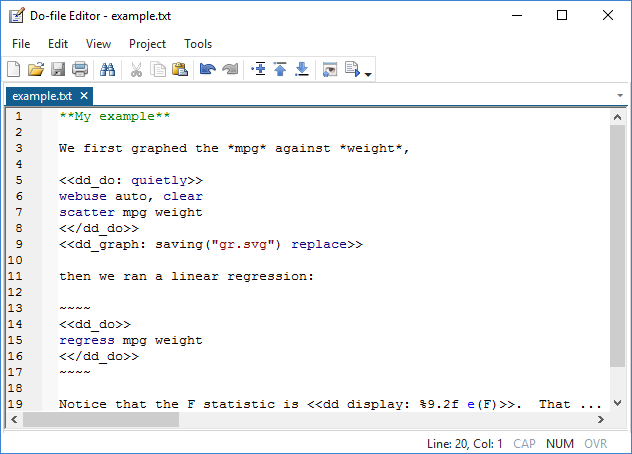
In Stata, you type

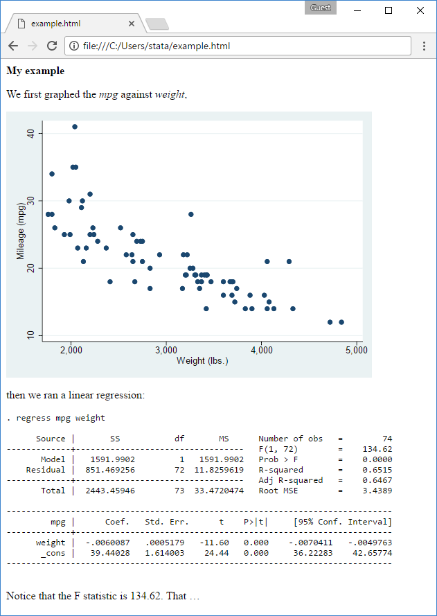
. dyndoc example.txt

and now you have a new file named example.html that, on the web, looks like this:

Learn more about the Markdown language at Wikipedia.

Learn more about our implementation at our Stata 15 Markdown & dynamic documents page.

dyndoc, by the way, stands for dynamic document. The Markdown file you create is dynamic in the sense that, should your data change, you can re-create the webpage by simply typing

. dyndoc filename

Back to highlights.

 

6. Nonlinear multilevel mixed-effects models

Nonlinear mixed-effects models are also known as nonlinear multilevel models and nonlinear hierarchical models. These models can be thought of in two ways. You can think of them as nonlinear models containing random effects. Or you can think of them as linear mixed-effects models in which some or all fixed and random effects enter nonlinearly. However you think of them, the overall error distribution is assumed to be Gaussian.

These models are popular because some problems are not, says their science, linear in the parameters. These models are popular in population pharmacokinetics, bioassays, and studies of biological and agricultural growth processes. For example, nonlinear mixed-effects models have been used to model drug absorption in the body, intensity of earthquakes, and growth of plants.

The new estimation command is named menl. It implements the popular-in-practice Lindstrom–Bates algorithm, which is based on the linearization of the nonlinear mean function with respect to fixed and random effects. Both maximum-likelihood and restricted maximum likelihood estimation methods are supported.

menl is easy to use. Single equations can be entered directly. Curly braces, { }, are used to enclose the parameters to be fit:

. menl weight = ({b1}+{U[plant]})/(1+exp(-(age-{b2})/{b3}))

To be estimated are b1, b2, and b3. U[plant] is a random intercept for each plant.

menl can also fit multistage or hierarchical specifications in which parameters can be defined at each level of hierarchy as functions of other model parameters and random effects, such as

. menl weight = {phi1:}/(1+exp(-(age-{phi2:})/{phi3:})),
                     define(phi1:{b1}+{U1[plant]})
                     define(phi2:{b2}+{U2[plant]})
                     define(phi3:{b3}+{U3[plant]})

This is the same model as the previous one except that b2 and b3 are allowed to vary across plants.

Several variance–covariance structures are available to model the dependence of random effects at the same level of hierarchy. If you wanted, you could have put dependence between U1, U2, and U3 in the above example.

Although not stated explicitly, there is a within-group error in the model. Flexible variance–covariance structures are available to model its heteroskedasticity and its within-group dependence. For instance, heteroskedasticity can be modeled as a power function of a covariate or even of predicted mean values, and dependence can be modeled using an autoregressive model of any order.

In addition to standard features, postestimation features also include prediction of random effects and their standard errors, prediction of parameters of interest defined in the model as functions of other model parameters and random effects, estimation of the overall within-cluster correlation matrix, and more.

See more at the Stata 15 Nonlinear multilevel mixed-effects models page.

Back to highlights.

 

7. Spatial autoregressive models (SAR)

Stata now fits spatial autoregressive (SAR) models, also known as simultaneous autoregressive models. The new spregress, spivregress, and spxtregress commands allow spatial lags of the dependent variable, spatial lags of the independent variables, and spatial autoregressive errors. Spatial lags are the spatial analog of time-series lags. Time-series lags are values of variables from recent times. Spatial lags are values from nearby areas.

The models are appropriate for area data, also known as areal data. Observations are called spatial units and might be countries, states, districts, counties, cities, postal codes, or city blocks. Or they might not be geographically based at all. They could be nodes of a social network. Spatial models estimate direct effects—the effects of areas on themselves—and estimate indirect or spillover effects—effects from nearby areas.

There is an entire new [SP] manual devoted to Stata's new SAR features. The commands are called the Sp commands. They can work with

1. shapefiles you obtain over the web along with data that you optionally provide, or
2. no shapefiles and data that you provide that contain the coordinates of the places, or
3. no shapefiles and no locations as would occur with social network data.

Here is how it works with shapefiles. You visited the U.S. Census website and downloaded the file tl_2016_us_county.zip. You now type

. unzipfile tl_2016_us_county.zip

. spshape2dta tl_2016_us_county

. use tl_2016_us_county       // file created by spshape2dta

. generate long fips = real(STATEFP + COUNTYFP)

. spset fips, modify replace

. save, replace

Next, you merge the newly created tl_2016_us.county.dta file with your analysis file:

. use analysis, clear 

. merge 1:1 fips using tl_2016_us_county, keep(match)

. save newdata

And you are ready to define spatial weighting matrices and fit models with spatial lags.

. spmatrix create contiguity W 

. spmatrix create idistance M

. spregress unemployment college, gs2sls dvarlag(W) 
                                  ivarlag(W:college) errorlag(M)

You just fit a model of unemployment on (1) college, (2) the spatial lag of the dependent variable, and (3) the spatial lag of college. The model has an autoregressive error too. Spatial lags of variables were calculated using W. Spatial lags of the error were calculated using M.

See more at the Stata 15 Spatial autoregressive models page.

Back to highlights.

 

8. Interval-censored parametric survival-time models

Stata's new stintreg command joins streg for fitting parametric survival models. stintreg fits models to interval-censored data. In interval-censored data, the time of failure is not exactly known. What is known are the times when subjects have not yet failed and later times when they have already failed.

stintreg fits exponential, Weibull, Gompertz, log-normal, log-logistic, and generalized gamma survival-time models. Both proportional-hazards and accelerated failure-time metrics are supported. Features include

• stratified estimation,
• flexible modeling of ancillary parameters, and
• robust, cluster–robust, bootstrap, and jackknife standard errors.

Survey-data estimation is supported via the svy prefix.

In addition to the usual features, postestimation features also include plots of survivor, hazard, and cumulative hazard functions; prediction of mean and median times; Cox–Snell and martingale-like residuals; and more.

See more at the Stata 15 Parametric survival models for interval-censored data page.

Back to highlights.

 

9. Finite mixture models (FMMs)

The new fmm: prefix command fits models when the data come from unobserved subpopulations. It can be used with seventeen Stata estimation commands.

Most users will use fmm to fit models in which parameters (coefficients, location, variance, scale, etc.) vary across subpopulations. In these models, the unobserved subpopulations are called classes. Say you are interested in fitting the model

. regress y x1 x2

but you believe there are three classes across which the parameters of the model might vary. Even though you have no variable recording the class membership, you can fit

. fmm 3: regress y x1 x2

Reported will be three linear regressions—one for each class—along with the model that predicts class membership.

fmm: can also be used with multiple estimation commands simultaneously when the classes might follow different models, such as

. fmm: (regress y x1 x2)
       (poisson y x1 x2 x3)

In this two-class example, reported will be a linear regression model for the first class, a Poisson regression for the second, and the model that predicts class membership.

Postestimation commands are available to (1) estimate each class's proportion in the overall population; (2) report marginal means of the outcome variables within class; and (3) predict probabilities of class membership and predicted outcomes.

See more at the Stata 15 Finite mixture models page.

Back to highlights.

 

10. Mixed logit models

Stata already fit multinomial logit models. Stata 15 can fit them in mixed form including random coefficients.

Random coefficients are of special interest to those fitting multinomial logistic models. They are a way around the Independence of the Irrelevant Alternatives (IIA) assumption. That assumption asserts that if you choose walking to work when your choices are walking, taking the bus, or driving, you would still choose walking even if one of the choices you did not choose were no longer available. You would still choose walking if the choice was between walking or driving. Humans sometimes behave differently.

IIA assumes that alternatives are independent after conditioning on the covariates. If that assumption is violated, the alternatives would be correlated. Random coefficients allow the alternatives to be correlated.

Researchers often use mixed models in the context of random-utility models and discrete choice analysis. Stata's new asmixlogit logit command supports a variety of random-coefficient distributions and allows the models that include case-specific variables.

See more at the Stata 15 Alternative-specific mixed logit regression page.

Back to highlights.

 

11. Nonparametric regression

Stata now fits nonparametric regressions. In these models, you do not specify a functional form. You specify variables and specify that you want to fit

y = g(x1, x2, ... xk) + ε

Fitted is g(). The method does not assume that g() is linear; it could just as well be

y = β1*x1 + β2*x2^2 + β3*x1*x2 + ... + ε

The method does not even assume that g() is linear in the parameters. It could just as well be

y = β1*x1^β2 + β3*cos(x2+x3) + ... + ε

To fit a model of y on x1, x2, and x3, type

. npregress kernel y x1 x2 x3 

Reported will be the averages of the partial derivatives of y with respect to x1, x2, and x3 and their standard errors, the last obtained by bootstrapping. The averages are calculated over the data. After fitting the model, you could obtain predicted values using predict.

Average derivatives are something like coefficients, or at least they would be if the model were linear, which it is not. Realize that the average derivatives in nonlinear models are not the derivatives at the average. You might want to know the derivative of y with respect to x1, x2, and x3 at the average values of the variables. You can use margins to obtain that:

. margins, dydx(x1 x2 x3) atmeans

Or perhaps you want the predicted values evaluated at specific points of interest,

. margins, at(x1=2 x2=3 x3=1) at(x1=2 x2=3 x3=2)

If you wanted x3 to be 1, 2, ..., 10, you could type

. margins, at(x1=2 x2=3 x3=1(1)10)

Then, you could type

. marginsplot

to graph this slice of the function.

By the way, margins not only makes calculations, it produces bootstrap standard errors for them, too.

See more at the Stata 15 Nonparametric regression page.

Back to highlights.

 

12. Power analysis for cluster randomized designs and regression models

Stata's existing power command performs power and sample-size (PSS) analysis. Its features now include PSS for linear regression and for cluster randomized designs (CRDs). And you can now add your own power and sample-size methods.

The new methods for linear regression include

• power oneslope, which performs PSS for a slope test in a simple linear regression. It computes sample size or power or the target slope given other study parameters.
• power rsquared, which performs PSS for an R-squared test in a multiple linear regression. An R-squared test is an F test for the coefficient of determination (R-squared). The test can be used to test the significance of all the coefficients, or it can be used to test a subset of them. In either case, power rsquared computes sample size or power or the target R-squared given other study parameters.
• power pcorr, which performs PSS for a partial-correlation test in a multiple linear regression. A partial-correlation test is an F test of the squared partial multiple correlation coefficient. The command computes sample size or power or the target squared partial correlation coefficient given other study parameters.

Stata 15 also now supports cluster randomized designs:

• In a CRD, groups of subjects (clusters) are randomized instead of individual subjects, meaning that the role of sample size is played by the number of clusters and the cluster size. The sample-size determination consists of the determination of the number of clusters given cluster size or the cluster size given the number of clusters. The CRD commands compute one of (1) the number of clusters, (2) cluster size, or (3) power, or minimum detectable effect size given other parameters. The commands have options to adjust for unequal cluster sizes.
• Five of the existing power methods are extended to support CRDs when you specify new option cluster. They are
  

  Command	Purpose in a CRD
  power onemean, cluster	One-sample mean test
  power oneproportion, cluster	One-sample proportion test
  power twomeans, cluster	Two-sample means test
  power twoproportions, cluster	Two-sample proportions test
  power logrank, cluster	Log-rank test

• For two-sample methods, you can also adjust for unequal numbers of clusters in the two groups.

As with all other power methods, the new methods allow you to specify multiple values of parameters and automatically produce tabular and graphical results.

The other new feature is that you can add your own PSS methods. It is easy to do. You write a program that computes sample size or power or effect size. The power command will do the rest for you. It will deal with the support of multiple values in options and with the automatic generation of graphs and tables of results.

See more at the Stata 15 feature pages for

• Power analysis for cluster randomized designs
• Power analysis for linear regression

Back to highlights.

 

13. Word and PDF documents

It is now just as easy to produce Word and PDF documents with Stata embedded results as it is to produce Excel worksheets. Lots of users loved putexcel in Stata 14. If you are among them, you will love the new putdocx and putpdf commands. They work just like putexcel. You can write do-files to create entire Word or PDF reports containing the latest results, tables, and graphs. You can automate reproducible reports.

The new putdocx command writes paragraphs, images, and tables to Word documents (.docx files). Images including Stata graphs and your organization's logo can be included. You can format the text objects, too. Included are font size, bold face, italics, custom tables, and the like.

See more at the Stata 15 pages for

• Create Word documents with embedded Stata results

• Create PDF files with embedded Stata results

Back to highlights.

 

14. Graph color transparency/opacity

Up until now, graph one thing on top of another, and the object on top covered up the object underneath. In the jargon of computer graphics, Stata's colors were fully opaque or, if you prefer, not at all transparent. Stata 15 lets you control the opacity of its colors.

Opacity is specified as a percent. By default, Stata's colors are 100 percent opaque.

You can specify opacity whenever you specify a color, such as in the mcolor() option, which controls the colors of markers. Rather than specifying green, you can specify green%50. Rather than specifying "0 255 0" (equivalent to green), you can specify "0 255 0%50". And you can specify %50 all by itself to make the default color 50 percent opaque. Do not specify %0, however. It is fully transparent, but it is also invisible.

Here is a graph in which we use %70 opacity:

See more at the Stata 15 Transparency in graphs page.

Back to highlights.

 

15. ICD-10-CM/PCS support

Stata 15 supports ICD-10-CM and ICD-10-PCS, the U.S. ICD-10 codes provided by the NCHS and CMS. Stata 15 supports the codes from version 2016 (starting October 2015), when they were mandated for use in the U.S, and supports all subsequent versions.

Stata began support of ICD in 1998, starting with ICD-9-CM version 16, and has supported every ICD-9 version thereafter. Stata has supported ICD-10 code versions since 2003.

Stata's ICD commands have grown since 1998 from being merely an automated list of valid codes and short phrases to being an entire data-management system for ICD codes. The system even includes the ability to manage multiple ICD versions in one dataset!

See more at the Stata 15 ICD-10-CM/PCS page.

Back to highlights.

 

16. Federal Reserve Economic Data (FRED) support

The St. Louis Federal Reserve makes available over 470,000 U.S. and international economic and financial time series to registered users. Registering is free and easy to do. The service is called FRED. It includes data from 84 sources, including the Federal Reserve, the Penn World Table, Eurostat, and the World Bank.

In Stata 15, you can use Stata's GUI to access and download FRED data. You can search or browse by category or release or source. You can click to select series of interest. Select 1 or select 100. When you click download, Stata will download them and combine them into a single, custom dataset in memory.

These same features are available from Stata's command line interface, too. The command is import fred. The command is convenient when you want to automate updating the 27 different series that you are tracking for a monthly report.

Stata can access FRED and ALFRED. ALFRED is FRED's historical archive data.

See more at the Stata 15 Easy import of Federal Reserve Economic Data page.

Back to highlights.

 

17. There's more, of course

Learn more about the above features at the Stata 15 features page and do not forget about

• Bayesian multilevel models
• Threshold regression
• Panel-data tobit with random coefficients
• Multilevel regression for interval-measured outcomes
• Multilevel tobit regression for censored outcomes
• Panel data cointegration tests
• Tests for multiple breaks in time series
• Multiple-group generalized SEM
• Heteroskedastic linear regression
• Poisson models with Heckman-style sample selection
• Panel-data nonlinear models with random coefficients
• Bayesian panel-data models
• Panel-data interval regression with random coefficients
• SVG export
• Bayesian survival models
• Zero-inflated ordered probit
• Add your own power and sample-size methods
• Bayesian sample-selection models
• And even more in statistics
• Stata in Swedish
• Improvements to the Do-file Editor
• Stream random-number generator
• Improvements for Java plugins
• More parallelization in Stata/MP

We also have 27 new videos about Stata 15 at our YouTube channel.