Nonlinear multilevel mixed-effects models
You have a model that is nonlinear in the parameters. Perhaps it is a model of tree growth and therefore asymptotes to a maximum value. Perhaps it is a model of serum concentrations of a drug that rise rapidly to a peak concentration and then decay exponentially. Easy enough, use nonlinear regression ([R] nl) to fit your model. But … what if you have repeated measures for each tree or repeated blood serum levels for each patient? You might want to account for the correlation within tree or patient. You might even believe that each tree has its own asymptotic growth. You need nonlinear mixed-effects models—also called nonlinear hierarchical models or nonlinear multilevel models.
The menl command, introduced in Stata 15, fits NLME models. Classical nonlinear models assume there is one observation per subject and that subjects are independent. You can think of NLME models as an extension of nonlinear models to the case where multiple measurements may be taken over a subject and these within-subject observations are usually correlated. You may also think of NLME models as a generalization of linear mixed-effects models where some or all random effects enter the model in a nonlinear fashion. Regardless of how you think of them, NLME models are used to describe a response variable as a (nonlinear) function of covariates, accounting for the correlation among observations on the same subject.
In this blog, I will walk you through several examples of fitting nonlinear mixed-effects models using menl. I will first fit a nonlinear model to the data on the growth of trees, ignoring the correlation among measurements on the same tree. I will then demonstrate different ways of accounting for this correlation and how to incorporate random effects into the model parameters to give the parameters tree-specific interpretation.
We have data (Draper and Smith 1998) on trunk circumference of five different orange trees where trunk circumference (in mm) was measured on seven different occasions, over roughly a four-year period of growth. We want to model the growth of orange trees. Let’s plot the data first.
. webuse orange
. twoway scatter circumf age, connect(L) ylabel(#6)
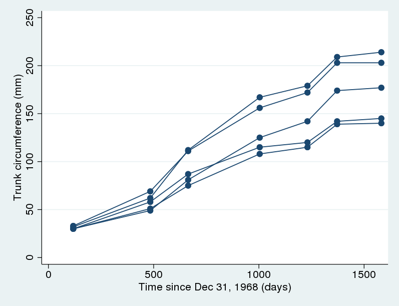
There is some variation in the growth curves, but the same overall shape is observed for all trees. In particular, the growth tends to level off toward the end. Pinheiro and Bates (2000) suggested the following nonlinear growth model for these data:
\[
{\mathsf{circumf}}_{ij}=\frac{\phi_{1}}{1+\exp\left\{ -\left( {\mathsf{age}}_{ij}-\phi_{2}\right)/\phi_{3}\right\}} + \epsilon_{ij}, \quad j=1,\dots,5; i=1,\dots,7
\]
Parameters of NLME models often have scientifically meaningful interpretations and form the basis of research questions. In this model, \(\phi_{1}\) is the average asymptotic trunk circumference of the trees as \(\mathsf{age}_{ij} \to \infty\), \(\phi_{2}\) is the average age at which the tree attains half the asymptotic trunk circumference \(\phi_{1}\) (half-life), and \(\phi_{3}\) is a scale parameter.
For now, let’s ignore the repercussions (less accurate estimates of uncertainty in parameter estimates, potentially less powerful tests of hypotheses, and less accurate interval estimates) of not accounting for the correlation and potential heterogeneity among the observations. Instead, we will treat all observations as being i.i.d.. We can use nl to fit the above model, but here we will use menl. (As of 15.1, menl no longer requires that you include random effects in the model specification.)
. menl circumf = {phi1}/(1+exp(-(age-{phi2})/{phi3})), stddeviations

Obtaining starting values:

NLS algorithm:

Iteration 0:   residual SS =  17480.234
Iteration 1:   residual SS =  17480.234

Computing standard errors:

Mixed-effects ML nonlinear regression           Number of obs     =         35
Log Likelihood = -158.39871
------------------------------------------------------------------------------
     circumf |      Coef.   Std. Err.      z    P>|z|     [95% Conf. Interval]
-------------+----------------------------------------------------------------
       /phi1 |   192.6876   20.24411     9.52   0.000     153.0099    232.3653
       /phi2 |   728.7564   107.2984     6.79   0.000     518.4555    939.0573
       /phi3 |   353.5337   81.47184     4.34   0.000     193.8518    513.2156
------------------------------------------------------------------------------

------------------------------------------------------------------------------
  Random-effects Parameters  |   Estimate   Std. Err.     [95% Conf. Interval]
-----------------------------+------------------------------------------------
                sd(Residual) |   22.34805   2.671102      17.68079    28.24734
------------------------------------------------------------------------------
The stddeviations option instructs menl to report the standard deviation of the error term instead of variance. Because one growth curve is used for all trees, the individual differences as depicted in the above graph are incorporated in the residuals, thus inflating the residual standard deviation.
We have multiple observations from the same tree that are likely to be correlated. One way to account for the dependence between observations within the same tree is by including a random effect, \(u_j\), shared by all the observations within the \(j\)th tree. Thus, our model becomes
$$
\mathsf{circumf}_{ij}=\frac{\phi_{1}}{1+\exp\left\{ -\left( \mathsf{age}_{ij}-\phi_{2}\right)/\phi_{3}\right\}} + u_j + \epsilon_{ij}, \quad j=1,\dots,5; i=1,\dots,7
$$
This model may be fit by typing
. menl circumf = {phi1}/(1+exp(-(age-{phi2})/{phi3}))+{U[tree]}, stddev

Obtaining starting values by EM:

Alternating PNLS/LME algorithm:

Iteration 1:    linearization log likelihood = -147.631786
Iteration 2:    linearization log likelihood = -147.631786

Computing standard errors:

Mixed-effects ML nonlinear regression           Number of obs     =         35
Group variable: tree                            Number of groups  =          5

                                                Obs per group:
                                                              min =          7
                                                              avg =        7.0
                                                              max =          7
Linearization log likelihood = -147.63179
------------------------------------------------------------------------------
     circumf |      Coef.   Std. Err.      z    P>|z|     [95% Conf. Interval]
-------------+----------------------------------------------------------------
       /phi1 |   192.2526   17.06127    11.27   0.000     158.8131    225.6921
       /phi2 |   729.3642   68.05493    10.72   0.000      595.979    862.7494
       /phi3 |    352.405   58.25042     6.05   0.000     238.2363    466.5738
------------------------------------------------------------------------------

------------------------------------------------------------------------------
  Random-effects Parameters  |   Estimate   Std. Err.     [95% Conf. Interval]
-----------------------------+------------------------------------------------
tree: Identity               |
                       sd(U) |   17.65093   6.065958      8.999985    34.61732
-----------------------------+------------------------------------------------
                sd(Residual) |    13.7099    1.76994      10.64497    17.65728
------------------------------------------------------------------------------
The fixed-effects estimates are similar in both models, but their standard errors are smaller in the above model. The residual standard deviation is also smaller because some of the individual differences are now being accounted for by the random effect. Let \(y_{sj}\) and \(y_{tj}\) be two observations on the \(j\)th tree. The inclusion of the random effect \(u_j\) implies that \({\rm Cov}(y_{sj},y_{tj}) > 0\) (in fact, it is equal to \({\rm Var}(u_j)\)). Therefore, \(u_j\) induces a positive correlation among any two observations within the same tree.
There is another way to account for the correlation among observations within a group. You can model the residual covariance structure explicitly using menl‘s rescovariance() option. For example, the above random-intercept nonlinear model is equivalent to a nonlinear marginal model with an exchangeable covariance matrix. Technically, the two models are equivalent only when the correlation of the within-group observations is positive.
. menl circumf = {phi1}/(1+exp(-(age-{phi2})/{phi3})),
    rescovariance(exchangeable, group(tree)) stddev

Obtaining starting values:

Alternating GNLS/ML algorithm:

Iteration 1:    log likelihood = -147.632441
Iteration 2:    log likelihood = -147.631786
Iteration 3:    log likelihood = -147.631786
Iteration 4:    log likelihood = -147.631786

Computing standard errors:

Mixed-effects ML nonlinear regression           Number of obs     =         35
Group variable: tree                            Number of groups  =          5

                                                Obs per group:
                                                              min =          7
                                                              avg =        7.0
                                                              max =          7
Log Likelihood = -147.63179
------------------------------------------------------------------------------
     circumf |      Coef.   Std. Err.      z    P>|z|     [95% Conf. Interval]
-------------+----------------------------------------------------------------
       /phi1 |   192.2526   17.06127    11.27   0.000     158.8131    225.6921
       /phi2 |   729.3642   68.05493    10.72   0.000      595.979    862.7494
       /phi3 |    352.405   58.25042     6.05   0.000     238.2363    466.5738
------------------------------------------------------------------------------

------------------------------------------------------------------------------
  Random-effects Parameters  |   Estimate   Std. Err.     [95% Conf. Interval]
-----------------------------+------------------------------------------------
Residual: Exchangeable       |
                          sd |   22.34987    4.87771      14.57155    34.28026
                        corr |   .6237137   .1741451      .1707327    .8590478
------------------------------------------------------------------------------
The fixed-effects portion of the output is identical in the two models. These two models also produce the same estimates of the marginal covariance matrix. You can verify this by running estat wcorrelation after each model. Although the two models are equivalent, by including a random effect on trees, we can not only account for the dependence of observations within trees, but also estimate between-tree variability and predict tree-specific effects after estimation.
The previous two models imply that the growth curves for all trees have the same shape and differ only by a vertical shift that equals \(u_j\). This may be too strong an assumption in practice. If we look back at the graph, we will notice there is an increasing variability in the trunk circumferences of trees as they approach their limiting height. Therefore, it may be more reasonable to allow \(\phi_1\) to vary between trees. This will also give our parameters of interest a tree-specific interpretation. That is, we assume
$$
\mathsf{circumf}_{ij}=\frac{\phi_{1}}{1+\exp\left\{ -\left( \mathsf{age}_{ij}-\phi_{2}\right)/\phi_{3}\right\}} + \epsilon_{ij}
$$
with
$$
\phi_1 = \phi_{1j} = \beta_1 + u_j
$$
You may interpret \(\beta_1\) as the average asymptotic height and \(u_j\) as a random deviation from the average that is specific to the \(j\)th tree. The above model may be fit as follows:
. menl circumf = ({b1}+{U1[tree]})/(1+exp(-(age-{phi2})/{phi3}))

Obtaining starting values by EM:

Alternating PNLS/LME algorithm:

Iteration 1:    linearization log likelihood = -131.584579

Computing standard errors:

Mixed-effects ML nonlinear regression           Number of obs     =         35
Group variable: tree                            Number of groups  =          5

                                                Obs per group:
                                                              min =          7
                                                              avg =        7.0
                                                              max =          7
Linearization log likelihood = -131.58458
------------------------------------------------------------------------------
     circumf |      Coef.   Std. Err.      z    P>|z|     [95% Conf. Interval]
-------------+----------------------------------------------------------------
         /b1 |    191.049   16.15403    11.83   0.000     159.3877    222.7103
       /phi2 |    722.556   35.15082    20.56   0.000     653.6616    791.4503
       /phi3 |   344.1624   27.14739    12.68   0.000     290.9545    397.3703
------------------------------------------------------------------------------

------------------------------------------------------------------------------
  Random-effects Parameters  |   Estimate   Std. Err.     [95% Conf. Interval]
-----------------------------+------------------------------------------------
tree: Identity               |
                     var(U1) |   991.1514   639.4636      279.8776    3510.038
-----------------------------+------------------------------------------------
               var(Residual) |   61.56371   15.89568      37.11466    102.1184
------------------------------------------------------------------------------
If desired, we can additionally model the within-tree error covariance structure using, for example, an exchangeable structure:
. menl circumf = ({b1}+{U1[tree]})/(1+exp(-(age-{phi2})/{phi3})),
    rescovariance(exchangeable)

Obtaining starting values by EM:

Alternating PNLS/LME algorithm:

Iteration 1:    linearization log likelihood = -131.468559
Iteration 2:    linearization log likelihood = -131.470388
Iteration 3:    linearization log likelihood = -131.470791
Iteration 4:    linearization log likelihood = -131.470813
Iteration 5:    linearization log likelihood = -131.470813

Computing standard errors:

Mixed-effects ML nonlinear regression           Number of obs     =         35
Group variable: tree                            Number of groups  =          5

                                                Obs per group:
                                                              min =          7
                                                              avg =        7.0
                                                              max =          7
Linearization log likelihood = -131.47081
------------------------------------------------------------------------------
     circumf |      Coef.   Std. Err.      z    P>|z|     [95% Conf. Interval]
-------------+----------------------------------------------------------------
         /b1 |   191.2005   15.59015    12.26   0.000     160.6444    221.7566
       /phi2 |   721.5232   35.66132    20.23   0.000     651.6283    791.4182
       /phi3 |   344.3675   27.20839    12.66   0.000     291.0401     397.695
------------------------------------------------------------------------------

------------------------------------------------------------------------------
  Random-effects Parameters  |   Estimate   Std. Err.     [95% Conf. Interval]
-----------------------------+------------------------------------------------
tree: Identity               |
                     var(U1) |   921.3895    582.735      266.7465    3182.641
-----------------------------+------------------------------------------------
Residual: Exchangeable       |
                         var |   54.85736   14.16704      33.06817    91.00381
                         cov |  -9.142893   2.378124     -13.80393   -4.481856
------------------------------------------------------------------------------
We did not specify option group() in the above because, in the presence of random effects, rescovariance() automatically determines the lowest-level group based on the specified random effects.
The NLME models we used so far are all linear in the random effect. In NLME models, random effects can enter the model nonlinearly, just like the fixed effects, and they often do. For instance, in addition to \(\phi_1\), we can let other parameters vary between trees and have their own random effects:
. menl circumf = {phi1:}/(1+exp(-(age-{phi2:})/{phi3:})),
    define(phi1:{b1}+{U1[tree]})
    define(phi2:{b2}+{U2[tree]})
    define(phi3:{b3}+{U3[tree]})
(output omitted)
The above model is too complicated for our data containing only five trees and is included purely for demonstration purposes. But from this example, you can see that the define() option is useful when you have a complicated nonlinear expression, and you would like to break it down into smaller pieces. Parameters specified within define() may also be predicted for each tree after estimation. For example, after we fit our model, we may wish to predict the asymptotic height, \(\phi_{1j}\), for each tree \(j\). Below, we are requesting to construct a variable named phi1 that contains the predicted values for the expression {phi1:}:
. predict (phi1 = {phi1:})
(output omitted)
If we had more trees, we could have also specified a covariance structure for these random effects as follows:
. menl circumf = {phi1:}/(1+exp(-(age-{phi2:})/{phi3:})),
    define(phi1:{b1}+{U1[tree]})
    define(phi2:{b2}+{U2[tree]})
    define(phi3:{b3}+{U3[tree]})
    covariance(U1 U2 U3, unstructured)
(output omitted)
I demonstrated only a few models in this article, but menl can do much more. For example, menl can incorporate higher levels of nesting such as three-level models (for example, repeated observations nested within trees and trees nested within planting zones). See [ME] menl for more examples.
References
Draper, N., and H. Smith. 1998. Applied Regression Analysis. 3rd ed. New York: Wiley.
Pinheiro, J. C., and D. M. Bates. 2000. Mixed-Effects Models in S and S-PLUS. New York: Springer.