Exploring results of nonparametric regression models
In his blog post, Enrique Pinzon discussed how to perform regression when we don’t want to make any assumptions about functional form—use the npregress command. He concluded by asking and answering a few questions about the results using the margins and marginsplot commands.
Recently, I have been thinking about all the different types of questions that we could answer using margins after nonparametric regression, or really after any type of regression. margins and marginsplot are powerful tools for exploring the results of a model and drawing many kinds of inferences. In this post, I will show you how to ask and answer very specific questions and how to explore the entire response surface based on the results of your nonparametric regression.
The dataset that we will use includes three covariates—continuous variables x1 and x2 and categorical variable a with three levels. If you would like to follow along, you can use these data by typing use http://www.stata.com/users/kmacdonald/blog/npblog.
Let’s first fit our model.
. npregress kernel y x1 x2 i.a, vce(boot, rep(10) seed(111))
(running npregress on estimation sample)

Bootstrap replications (10)
----+--- 1 ---+--- 2 ---+--- 3 ---+--- 4 ---+--- 5
..........

Bandwidth
------------------------------------
             |      Mean     Effect
-------------+----------------------
          x1 |  .4795422   1.150255
          x2 |  .7305017    1.75222
           a |  .3872428   .3872428
------------------------------------

Local-linear regression                    Number of obs      =          1,497
Continuous kernel : epanechnikov           E(Kernel obs)      =            524
Discrete kernel   : liracine               R-squared          =         0.8762
Bandwidth         : cross validation
------------------------------------------------------------------------------
             |   Observed   Bootstrap                          Percentile
           y |   Estimate   Std. Err.      z    P>|z|     [95% Conf. Interval]
-------------+----------------------------------------------------------------
Mean         |
           y |   15.64238   .3282016    47.66   0.000     15.17505    16.38781
-------------+----------------------------------------------------------------
Effect       |
          x1 |   3.472485   .2614388    13.28   0.000     2.895202    3.846091
          x2 |   4.143544   .2003619    20.68   0.000     3.830656    4.441306
             |
           a |
   (2 vs 1)  |   1.512241   .2082431     7.26   0.000     .9880627    1.717007
   (3 vs 1)  |  -10.23723   .2679278   -38.21   0.000     -10.6352   -9.715858
------------------------------------------------------------------------------
Note: Effect estimates are averages of derivatives for continuous covariates
      and averages of contrasts for factor covariates.
Enrique discussed interpretation of these results in his blog, so I will not focus on it here. I should, however, point out that because my goal is to show you how to use margins, I used only 10 bootstrap replications (a ridiculously small number) when estimating standard errors. In real research, you would certainly want to use more replications both with the npregress command and the margins commands that follow.
The npregress output includes estimates of the effects of x1, x2, and the levels of a on our outcome, but these estimates are probably not enough to answer some of the important questions that we want to address in our research.
Below, I will first show you how you can explore the nonlinear response surface—the expected value of y at different combinations of x1, x2, and a. For instance, suppose your outcome variable is the response to a drug, and you want to know the expected value for a female whose weight is 150 pounds and whose cholesterol level is 220 milligrams per deciliter. What about for a male with the same characteristics? How do these expectations change across a range of weights and cholesterol levels?
I will also demonstrate how to answer questions about population averages, counterfactuals, treatment effects, and more. These are exactly the types of questions that policy makers ask. How, on average, does a variable affect the population they are interested in? For instance, suppose your outcome variable is income of individuals in their 20s. What is the expected value of income for this group, the population average? What is the expected value if, instead of having their observed education level, they were all high school graduates? What if they were all college graduates? What is the difference in these values—the effect of college education?
These are just a few examples of the types of questions that you could answer. I will continue with variable names x1, x2, and a below, but you can imagine relevant questions for your research.
Exploring the response surface
Let’s start at the beginning. We might want to know the expected value of the outcome at one specific point. To get the expected value of y when a=1, x1=2, and x2=5, we can type
. margins 1.a, at(x1=2 x2=5) reps(10)
(running margins on estimation sample)

Bootstrap replications (10)
----+--- 1 ---+--- 2 ---+--- 3 ---+--- 4 ---+--- 5
..........

Adjusted predictions                            Number of obs     =      1,497
                                                Replications      =         10

Expression   : mean function, predict()
at           : x1              =           2
               x2              =           5

------------------------------------------------------------------------------
             |   Observed   Bootstrap                          Percentile
             |     Margin   Std. Err.      z    P>|z|     [95% Conf. Interval]
-------------+----------------------------------------------------------------
         1.a |   12.66575   .4428049    28.60   0.000     11.57809     13.0897
------------------------------------------------------------------------------
We predict that y=12.7 at this point.
We could evaluate it at another point, say, a=2, x1=2, and x2=5.
. margins 2.a, at(x1=2 x2=5) reps(10)
(running margins on estimation sample)

Bootstrap replications (10)
----+--- 1 ---+--- 2 ---+--- 3 ---+--- 4 ---+--- 5
..........

Adjusted predictions                            Number of obs     =      1,497
                                                Replications      =         10

Expression   : mean function, predict()
at           : x1              =           2
               x2              =           5

------------------------------------------------------------------------------
             |   Observed   Bootstrap                          Percentile
             |     Margin   Std. Err.      z    P>|z|     [95% Conf. Interval]
-------------+----------------------------------------------------------------
         2.a |   14.80935   .6774548    21.86   0.000     13.48154    15.98991
------------------------------------------------------------------------------
With a=2, the expected value of y is now 14.8.
What if our interest is in the effect of going from a=1 to a=2 when x1=2 and x2=5? That is just a contrast—the difference in our two previous results. Using the r. contrast operator with margins, we can perform a hypothesis test of whether these two values are the same.
. margins r(1 2).a, at(x1=2 x2=5) reps(10)
(running margins on estimation sample)

Bootstrap replications (10)
----+--- 1 ---+--- 2 ---+--- 3 ---+--- 4 ---+--- 5
..........
Contrasts of predictive margins
                                                Number of obs     =      1,497
                                                Replications      =         10

Expression   : mean function, predict()
at           : x1              =           2
               x2              =           5

------------------------------------------------
             |         df        chi2     P>chi2
-------------+----------------------------------
           a |          1       27.58     0.0000
------------------------------------------------

--------------------------------------------------------------
             |   Observed   Bootstrap          Percentile
             |   Contrast   Std. Err.     [95% Conf. Interval]
-------------+------------------------------------------------
           a |
   (2 vs 1)  |   2.143598   .4081472      1.335078    2.523469
--------------------------------------------------------------
The confidence interval for the difference does not include 0. Using a 5% significance level, we find that the expected value is significantly different for these two points of interest.
But we might be interested in more than these two points. Let’s continue holding x2 to 5 and look at a range of values for x1. And let’s estimate the expected values across all three levels of a. In other words, let’s look at a slice of the 3-dimensional response surface (at x2=5) and examine the relationship between the other two variables.
. margins a, at(x1=(1(1)4) x2=5) reps(10)
(running margins on estimation sample)

Bootstrap replications (10)
----+--- 1 ---+--- 2 ---+--- 3 ---+--- 4 ---+--- 5
..........

Adjusted predictions                            Number of obs     =      1,497
                                                Replications      =         10

Expression   : mean function, predict()

1._at        : x1              =           1
               x2              =           5

2._at        : x1              =           2
               x2              =           5

3._at        : x1              =           3
               x2              =           5

4._at        : x1              =           4
               x2              =           5

------------------------------------------------------------------------------
             |   Observed   Bootstrap                          Percentile
             |     Margin   Std. Err.      z    P>|z|     [95% Conf. Interval]
-------------+----------------------------------------------------------------
       _at#a |
        1 1  |   9.075231   2.017476     4.50   0.000     5.984868    12.61052
        1 2  |   14.35551   2.488854     5.77   0.000     9.944582    17.73349
        1 3  |  -.2925357   1.499151    -0.20   0.845    -1.991074    2.248606
        2 1  |   12.66575   .3285203    38.55   0.000     11.93955    13.03459
        2 2  |   14.80935   .8713405    17.00   0.000     12.92743    15.75046
        2 3  |    1.82419   .5384259     3.39   0.001     .6331934    2.422084
        3 1  |    17.1207   .2446792    69.97   0.000     16.89714    17.61579
        3 2  |   17.28286   .3536435    48.87   0.000     16.78102    17.89018
        3 3  |     6.2364   .2689665    23.19   0.000     5.695041      6.5686
        4 1  |   21.29851   .1441116   147.79   0.000     21.05866    21.54149
        4 2  |   18.96943   .2000661    94.82   0.000     18.50348    19.24232
        4 3  |   11.45945   .2037134    56.25   0.000     11.05172    11.69403
------------------------------------------------------------------------------
Better yet, let’s plot these values.
. marginsplot
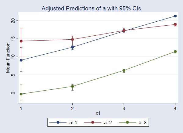
We find that when x2=5, the expected value of y increases as x1 increases, and the expected value is lower for a=3 than for a=1 and a=2 across all levels of x1.
But is this pattern the same for other values of x2?
We have only three covariates. So we can explore the entire response surface easily. Let’s look at additional slices at other values of x2. Here’s the command:
. margins a, at(x1=(1(1)4) x2=(2 5 8)) reps(10)
This produces a lot of output, so I won’t show it. But here is the graph
. marginsplot, bydimension(x2) byopts(cols(3))
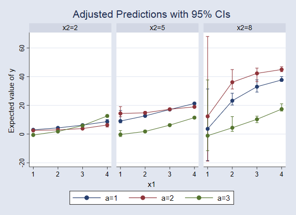
We can now see that the response surface changes as x2 changes. When x2=2, the expected value of y increases slightly as x1 increases, but there is almost no difference among the levels of a. For x2=8, the differences among levels of a are more pronounced and appear to have a different pattern, increasing with x1 and then beginning to level off.
Earlier, we typed r(1 2).a to test for a difference in expected values when a=1 and a=2. Similarly, we could type r(1 3).a to compare a=1 with a=3. We could make both of those comparisons by simply typing r.a. And we can do this across a range of values of x1 and x2. We just change a to r.a in our previous margins command.
. margins r.a, at(x1=(1(1)4) x2=(2 5 8)) reps(10)
(running margins on estimation sample)

Bootstrap replications (10)
----+--- 1 ---+--- 2 ---+--- 3 ---+--- 4 ---+--- 5
..........
Contrasts of predictive margins
                                                Number of obs     =      1,497
                                                Replications      =         10

Expression   : mean function, predict()

1._at        : x1              =           1
               x2              =           2

2._at        : x1              =           1
               x2              =           5

(output omitted)

--------------------------------------------------------------
             |   Observed   Bootstrap          Percentile
             |   Contrast   Std. Err.     [95% Conf. Interval]
-------------+------------------------------------------------
       a@_at |
(2 vs 1)  1  |  -.4316907   .2926308     -.6839362    .2414861
(2 vs 1)  2  |   5.280281   .7986439      3.821515    6.316996
(2 vs 1)  3  |   8.716763   9.371615     -7.472455    19.98571
(2 vs 1)  4  |  -1.388968   .1918396     -1.756544   -1.110874
(2 vs 1)  5  |   2.143598   .4487908      1.075932    2.563385
(2 vs 1)  6  |   12.88835   4.544753      6.060425    20.50299
(2 vs 1)  7  |  -2.384115   .2101401     -2.736413   -2.082235
(2 vs 1)  8  |   .1621524   .3430663     -.3141147    .6630604
(2 vs 1)  9  |   9.285226   1.292208      7.300806    10.96053
(2 vs 1) 10  |  -2.355113   .5453254     -2.893817   -1.346538
(2 vs 1) 11  |  -2.329082   .2355506     -2.717465   -1.844513
(2 vs 1) 12  |   7.264358   1.152335      5.603027    9.361632
(3 vs 1)  1  |  -3.622857   .6110854     -4.141618   -2.277811
(3 vs 1)  2  |  -9.367766   .9618594     -10.86855   -8.056798
(3 vs 1)  3  |  -4.751952    8.78832     -14.17876     12.3299
(3 vs 1)  4  |  -2.500585   .2942087     -2.999642   -2.113881
(3 vs 1)  5  |  -10.84156   .3575732     -11.46529    -10.4761
(3 vs 1)  6  |  -18.84966   2.783479     -21.87325   -11.56521
(3 vs 1)  7  |  -.3080399   .1685899     -.7749465   -.1793496
(3 vs 1)  8  |   -10.8843    .271959     -11.28382   -10.48519
(3 vs 1)  9  |  -22.70852   1.147957     -23.26496   -19.51463
(3 vs 1) 10  |   3.922399   .6064593      2.976073    4.793276
(3 vs 1) 11  |  -9.839058   .2572868     -10.13578   -9.339336
(3 vs 1) 12  |  -20.31851   1.294548      -22.1466   -17.29554
--------------------------------------------------------------
The legend at the top of the output tells us that 1._at corresponds to x1=1 and x2=2. The values parentheses, such as (2 vs 1), at the first of each line in the table tell us which values of a are compared in that line. Thus, the first line in the table provides a test comparing expected values of y for a=2 versus a=1 when x1=1 and x2=2. Admittedly, this is a lot to look at, and it is probably easier to interpret with a graph. We use marginsplot to graph these differences with their confidence intervals. This time, let’s use the yline(0) option to add a reference line at 0. This allows us to perform the test visually by checking whether the confidence interval for the difference includes 0.
. marginsplot, bydimension(x2) byopts(cols(3)) yline(0)
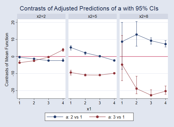
In this case, some of the confidence intervals are so narrow that they are hard to see. If we look closely at the blue point on the far left, we see that the confidence interval for the difference comparing a=2 versus a=1 when x1=1 and x2=2 (corresponding to the first line in the output above) does include 0. This indicates that there is not a significant difference in these expected values. We can examine each of the other points and confidence intervals in the same way. For example, looking at the red line and points in the third panel, we see that the effect of moving from a=1 to a=3 is negative and significantly different from 0 for x1 values of 2, 3, and 4. When x1 is 1, the point estimate of the effect is still negative, but that effect is not significantly different from 0 at the 95% level. But recall that we should dramatically increase the number of bootstrap replicates to make any real claims about confidence intervals.
So far, we have compared both a=2 with a=1 and a=3 with a=1. But we are not limited to making comparisons with a=1. We could compare 1 with 2 and 2 with 3, which often makes more sense if levels of a have a natural ordering. To do this, we just replace r. with ar. in our margins command. I won’t show that output, but you have the data and can try it if you like.
Population-averaged results
So far, we have talked about evaluating individual points on your response surface and how to perform tests comparing expected values at those points. Now, let’s switch gears and talk about population-averaged results.
We are going to need the dataset to be representative of the population. If that is not true of your data, you will want to stop with the analyses we did above. We will assume our data are representative so that we can answer a variety of questions based on average predictions.
First, what is the overall expected population mean from this response surface?
. margins, reps(10)
(running margins on estimation sample)

Bootstrap replications (10)
----+--- 1 ---+--- 2 ---+--- 3 ---+--- 4 ---+--- 5
..........

Predictive margins                              Number of obs     =      1,497
                                                Replications      =         10

Expression   : mean function, predict()

------------------------------------------------------------------------------
             |   Observed   Bootstrap                          Percentile
             |     Margin   Std. Err.      z    P>|z|     [95% Conf. Interval]
-------------+----------------------------------------------------------------
       _cons |   15.64238    .318746    49.07   0.000     15.34973    16.24543
------------------------------------------------------------------------------
Whatever the process was that generated this, we believe 15.6 is the expected value in the population and [15.3, 16.2] is the confidence intervals for it.
Do the population averages differ when we first set everyone to have a=1, then set everyone to have a=2, and finally set everyone to have a=3? Let’s look at the expected means for all three.
. margins a, reps(10)
(running margins on estimation sample)

Bootstrap replications (10)
----+--- 1 ---+--- 2 ---+--- 3 ---+--- 4 ---+--- 5
..........

Predictive margins                              Number of obs     =      1,497
                                                Replications      =         10

Expression   : mean function, predict()

------------------------------------------------------------------------------
             |   Observed   Bootstrap                          Percentile
             |     Margin   Std. Err.      z    P>|z|     [95% Conf. Interval]
-------------+----------------------------------------------------------------
           a |
          1  |   18.39275   .4847808    37.94   0.000     17.63322    19.31199
          2  |   19.90499   .6840056    29.10   0.000     18.17305    20.57171
          3  |   8.155515   .3239624    25.17   0.000      7.59187     8.70898
------------------------------------------------------------------------------
We get 18.4, 19.9, and 8.2. They sure don’t look the same. Let’s test them.
. margins r.a, reps(10)
(running margins on estimation sample)

Bootstrap replications (10)
----+--- 1 ---+--- 2 ---+--- 3 ---+--- 4 ---+--- 5
..........
Contrasts of predictive margins
                                                Number of obs     =      1,497
                                                Replications      =         10

Expression   : mean function, predict()

------------------------------------------------
             |         df        chi2     P>chi2
-------------+----------------------------------
           a |
   (2 vs 1)  |          1       17.10     0.0000
   (3 vs 1)  |          1      618.86     0.0000
      Joint  |          2     1337.66     0.0000
------------------------------------------------

--------------------------------------------------------------
             |   Observed   Bootstrap          Percentile
             |   Contrast   Std. Err.     [95% Conf. Interval]
-------------+------------------------------------------------
           a |
   (2 vs 1)  |   1.512241   .3656855      1.051265    2.016566
   (3 vs 1)  |  -10.23723   .4115157     -10.82644     -9.4265
--------------------------------------------------------------
In the causal-inference or treatment-effects literature, the means would be considered potential-outcome means, and these differences would be the average treatment effects of a multivalued treatment. Here the average treatment effect of a=2 (compared with a=1) is 1.5.
We saw in the previous section that differences in expected values for levels of a varied across values of x2. Let’s estimate the potential-outcome means and treatment effects of a at different values of x2. Notice that these are still population averages because, unlike in the previous section, we are not setting x1 to any specific value. Instead, predictions use the observed values of x1 in the data.
. margins a, at(x2=(2 5 8)) reps(10)
(running margins on estimation sample)

Bootstrap replications (10)
----+--- 1 ---+--- 2 ---+--- 3 ---+--- 4 ---+--- 5
..........

Predictive margins                              Number of obs     =      1,497
                                                Replications      =         10

Expression   : mean function, predict()

1._at        : x2              =           2

2._at        : x2              =           5

3._at        : x2              =           8

------------------------------------------------------------------------------
             |   Observed   Bootstrap                          Percentile
             |     Margin   Std. Err.      z    P>|z|     [95% Conf. Interval]
-------------+----------------------------------------------------------------
       _at#a |
        1 1  |   3.707771   .6552861     5.66   0.000     4.619393     6.70335
        1 2  |   1.340815   .9491373     1.41   0.158     2.077606    5.010682
        1 3  |   3.677883    .935561     3.93   0.000      4.33317    7.380818
        2 1  |   17.16092     .27028    63.49   0.000      16.8047    17.75164
        2 2  |   17.22508   .1993421    86.41   0.000     16.91111    17.57034
        2 3  |   6.933778   .1929387    35.94   0.000     6.751693    7.332845
        3 1  |   30.61528   .9961323    30.73   0.000     28.66033    31.88367
        3 2  |   40.17685   1.687315    23.81   0.000     36.18359    41.73811
        3 3  |   10.97667   .9771489    11.23   0.000     9.510952    12.59133
------------------------------------------------------------------------------
Instead of looking at the output, let’s graph these potential-outcome means.
. marginsplot
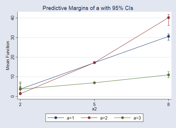
The effect of a increases as x2 increases. The effect is largest when x2=8.
Now, we can test for differences at each level of x2
. margins r.a, at(x2=(2 5 8)) reps(10)
(running margins on estimation sample)

Bootstrap replications (10)
----+--- 1 ---+--- 2 ---+--- 3 ---+--- 4 ---+--- 5
..........
Contrasts of predictive margins
                                                Number of obs     =      1,497
                                                Replications      =         10

Expression   : mean function, predict()

1._at        : x2              =           2

2._at        : x2              =           5

3._at        : x2              =           8

------------------------------------------------
             |         df        chi2     P>chi2
-------------+----------------------------------
       a@_at |
 (2 vs 1) 1  |          1       51.80     0.0000
 (2 vs 1) 2  |          1        0.13     0.7184
 (2 vs 1) 3  |          1       43.16     0.0000
 (3 vs 1) 1  |          1        0.01     0.9322
 (3 vs 1) 2  |          1      834.54     0.0000
 (3 vs 1) 3  |          1      245.45     0.0000
      Joint  |          6     2732.16     0.0000
------------------------------------------------

--------------------------------------------------------------
             |   Observed   Bootstrap          Percentile
             |   Contrast   Std. Err.     [95% Conf. Interval]
-------------+------------------------------------------------
       a@_at |
 (2 vs 1) 1  |  -2.366956   .3288861     -2.737075   -1.466043
 (2 vs 1) 2  |   .0641596   .1779406      -.224935    .3180577
 (2 vs 1) 3  |   9.561575   1.455483      6.847319    11.96769
 (3 vs 1) 1  |  -.0298883   .3513035     -.6345751    .4584875
 (3 vs 1) 2  |  -10.22714   .3540221     -10.89414   -9.808236
 (3 vs 1) 3  |  -19.63861   1.253521     -21.45499    -18.0223
--------------------------------------------------------------
Again, let’s look at the graph.
. marginsplot
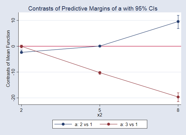
The difference in means when a=3 and a=1, the treatment effect, is not significant when x2=2. Neither is the effect of a=2 versus a=1 when x2=5. All the other effects are significantly different from 0.
Conclusion
In this blog, we have explored the response surface of a nonlinear function, we have estimated a variety of population averages based on our nonparametric regression model, and we have performed several tests comparing expected values at specific points of the response surface and tests comparing population averages. Yet, we have only scratched the surface of the types of estimates and tests you can obtain using margins after npregress. There are additional contrasts operators that will allow you to test differences from a grand mean, differences from means of previous or subsequent levels, and more. See [R] contrast for details of the available contrast operators. You can also use marginsplot to see the results of margins commands from different angles. For instance, if we type marginsplot, bydimension(x1) instead of marginsplot, bydimension(x2), we see our nonlinear response surface from a different perspective. See [R] marginsplot for details and examples of this command.
Whether you use nonparametric regression or another model, margins and marginsplot are the solution for exploring the results, making inferences, and understanding relationships among the variables you are studying.