Calculating power using Monte Carlo simulations, part 2: Running your simulation using power
In my last post, I showed you how to calculate power for a t test using Monte Carlo simulations. In this post, I will show you how to integrate your simulations into Stata’s power command so that you can easily create custom tables and graphs for a range of parameter values.
Statisticians rarely compute power for a single set of assumptions when planning a scientific study. We typically calculate power for a range of parameter values and choose a realistic set of assumptions that is financially and logistically feasible. For example, below I’ve used power onemean to calculate power for sample sizes ranging from 50 to 100 in increments of 10. The table displays the assumed parameter values, including the alpha level, the means under the null and alternative hypotheses, the standardized difference between the means (delta), the standard deviation, and power for each sample size.
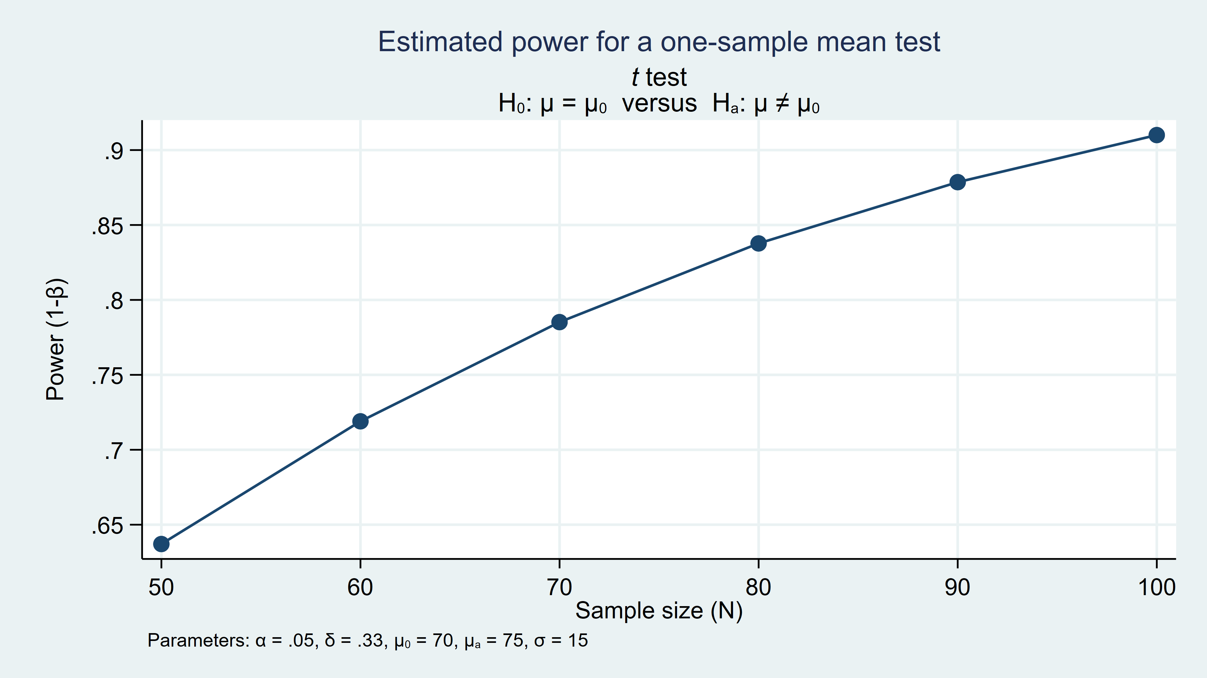
. power onemean 70 75, n(50(10)100) sd(15) alpha(0.05)

Estimated power for a one-sample mean test
t test
Ho: m = m0  versus  Ha: m != m0

  +---------------------------------------------------------+
  |   alpha   power       N   delta      m0      ma      sd |
  |---------------------------------------------------------|
  |     .05   .6371      50   .3333      70      75      15 |
  |     .05    .719      60   .3333      70      75      15 |
  |     .05   .7852      70   .3333      70      75      15 |
  |     .05   .8377      80   .3333      70      75      15 |
  |     .05   .8786      90   .3333      70      75      15 |
  |     .05     .91     100   .3333      70      75      15 |
  +---------------------------------------------------------+
I’ve also used the graph option below to plot power over the range of sample sizes. I can then use the table and graph to select a sample size that meets the power requirements for my study.
. power onemean 70 75, n(50(10)100) sd(15) alpha(0.05) graphFigure 1: Estimated power for n = 50 to 100 in increments of 10
In addition to sample size, the power commands allow you to enter a range of values for other parameters such as the standard deviation, the means, or the alpha level. And power will create tables and graphs of the results.
You can also add your own methods to the power suite of commands. Let’s add the t test simulation program from my last post to power to see how this works.
Recall from my last post that we created a program called simttest to calculate power for a t test. The program accepts five input parameters, creates a pseudo-random dataset assuming the alternative hypothesis, tests the null hypothesis, and returns the results of the hypothesis test.
capture program drop simttest
program simttest, rclass
    version 15.1
    syntax, n(integer)          ///  Sample size
          [ alpha(real 0.05)    ///  Alpha level
            m0(real 0)          ///  Mean under the null
            ma(real 1)          ///  Mean under the alternative
            sd(real 1) ]        //   Standard deviation
    drawnorm y, n(`n') means(`ma') sds(`sd') clear
    ttest y = `m0'
    return scalar reject = (r(p)<`alpha')
end
We used simulate to run the program many times and save the results to a variable named reject.
. simulate reject=r(reject), reps(100) seed(12345):
>         simttest, n(100) m0(70) ma(75) sd(15) alpha(0.05)

      command:  simttest, n(100) m0(70) ma(75) sd(15) alpha(0.05)
       reject:  r(reject)

Simulations (100)
----+--- 1 ---+--- 2 ---+--- 3 ---+--- 4 ---+--- 5
..................................................    50
..................................................   100
Then, we calculated power as the proportion of times that the null hypothesis was rejected.
. summarize reject

    Variable |        Obs        Mean    Std. Dev.       Min        Max
-------------+---------------------------------------------------------
      reject |        100         .91    .2876235          0          1

. local power = r(mean)

. display "power = `power'"
power = .91
You can add this simulation method to power by creating a program named power_cmd_mymethod, where mymethod is the name of the power command. Let’s call the program power_cmd_simttest.
The code block below defines power_cmd_simttest. Note how similar it is to our simttest program. It begins with capture program drop, then program, and version 15.1. Next, we define the input parameters using syntax just as we did in simttest. Here I have added a new input parameter called reps(), which is the number of repetitions for the simulation.
capture program drop power_cmd_simttest
program power_cmd_simttest, rclass
    version 15.1

    // DEFINE THE INPUT PARAMETERS AND THEIR DEFAULT VALUES
    syntax, n(integer)          ///  Sample size
          [ alpha(real 0.05)    ///  Alpha level
            m0(real 0)          ///  Mean under the null
            ma(real 1)          ///  Mean under the alternative
            sd(real 1)          ///  Standard deviation
            reps(integer 100)]  //   Number of repetitions

    // GENERATE THE RANDOM DATA AND TEST THE NULL HYPOTHESIS
    quietly simulate reject=r(reject), reps(`reps'):    ///
                     simttest, n(`n') m0(`m0') ma(`ma') sd(`sd') alpha(`alpha')
    quietly summarize reject

    // RETURN RESULTS
    return scalar power = r(mean)
    return scalar N = `n'
    return scalar alpha = `alpha'
    return scalar m0 = `m0'
    return scalar ma = `ma'
    return scalar sd = `sd'
end
The middle section of the program runs the simulation and summarizes the results. Both simulate and summarize are preceded by quietly, which suppresses the display of their output. Here simulate runs the program simttest and saves the results to the variable reject just as it did before. Note that all the input parameters in both simulate and simttest are local macros defined with syntax. summarize calculates the mean of reject and stores it in the scalar r(mean).
The bottom section of the code block returns power and the other parameters. The scalar power returns the mean of the variable reject, and the other parameters are simply local macros passed through from syntax.
Now you can run the simulation by typing power simttest.
. power simttest, n(100) m0(70) ma(75) sd(15)

Estimated power
Two-sided test

  +-------------------------------------------------+
  |   alpha   power       N      m0      ma      sd |
  |-------------------------------------------------|
  |     .05     .91     100      70      75      15 |
  +-------------------------------------------------+
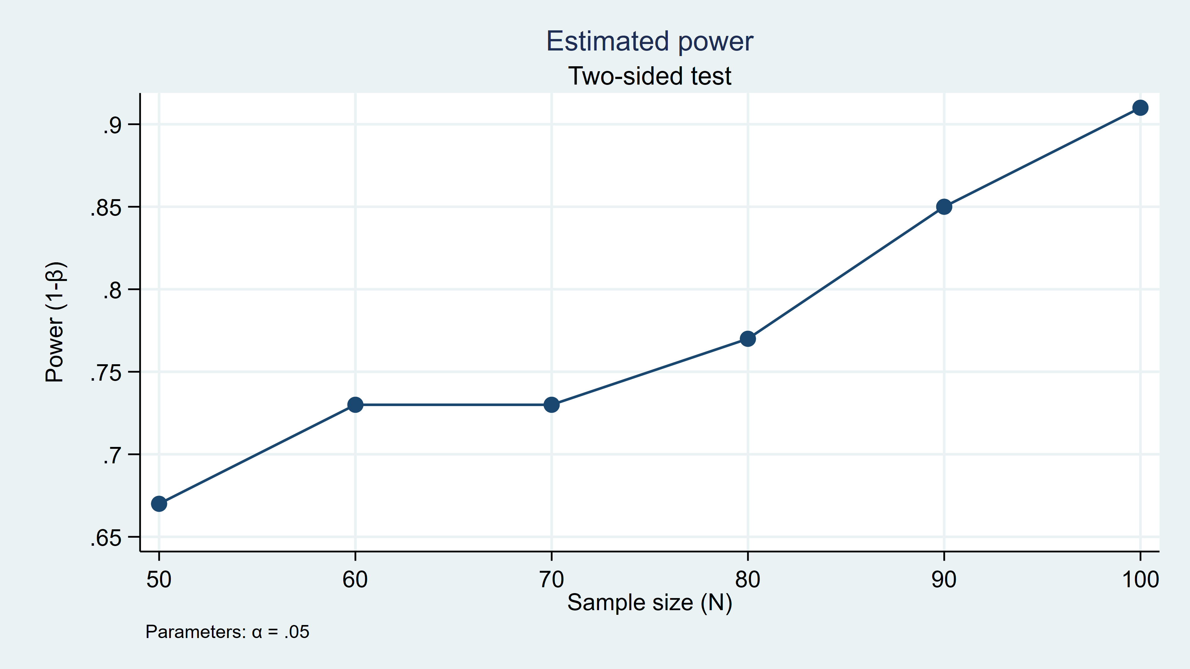
It worked! You can even make a table and graph for a range of sample sizes.
. power simttest, n(50(10)100) m0(70) ma(75) sd(15) table graph

Estimated power
Two-sided test

  +-------------------------------------------------+
  |   alpha   power       N      m0      ma      sd |
  |-------------------------------------------------|
  |     .05     .67      50      70      75      15 |
  |     .05     .73      60      70      75      15 |
  |     .05     .73      70      70      75      15 |
  |     .05     .77      80      70      75      15 |
  |     .05     .85      90      70      75      15 |
  |     .05     .91     100      70      75      15 |
  +-------------------------------------------------+
Figure 2: Simulated power for n = 50 to 100 in increments of 10
You could stop here if you wanted to consider only a range of sample sizes. But you will need to write one more small program if you wish to enter a range of values for the other parameters such as m0, ma, and sd. The program must be named power_cmd_mymethod_init, so we will name our program power_cmd_simttest_init.
The code block below defines power_cmd_simttest_init and begins with capture program drop and program just as our other programs. Note that the program definition begins with the option sclass. The line sreturn local pss_colnames initializes columns in the output table for the parameters listed in double quotes. The line sreturn local pss_numopts allows you to specify numlists for the parameters placed in double quotes.
capture program drop power_cmd_simttest_init
program power_cmd_simttest_init, sclass
    sreturn local pss_colnames "m0 ma sd"
    sreturn local pss_numopts  "m0 ma sd"
end
Now you can use power simttest to calculate power for a range of means assuming different alternative hypotheses. You can even do this for different sample sizes.
. power simttest, n(75 100) m0(70) ma(72(1)75) sd(15) reps(1000)

Estimated power
Two-sided test

  +-------------------------------------------------+
  |   alpha   power       N      m0      ma      sd |
  |-------------------------------------------------|
  |     .05    .212      75      70      72      15 |
  |     .05    .411      75      70      73      15 |
  |     .05    .611      75      70      74      15 |
  |     .05    .789      75      70      75      15 |
  |     .05    .265     100      70      72      15 |
  |     .05     .51     100      70      73      15 |
  |     .05    .761     100      70      74      15 |
  |     .05    .905     100      70      75      15 |
  +-------------------------------------------------+
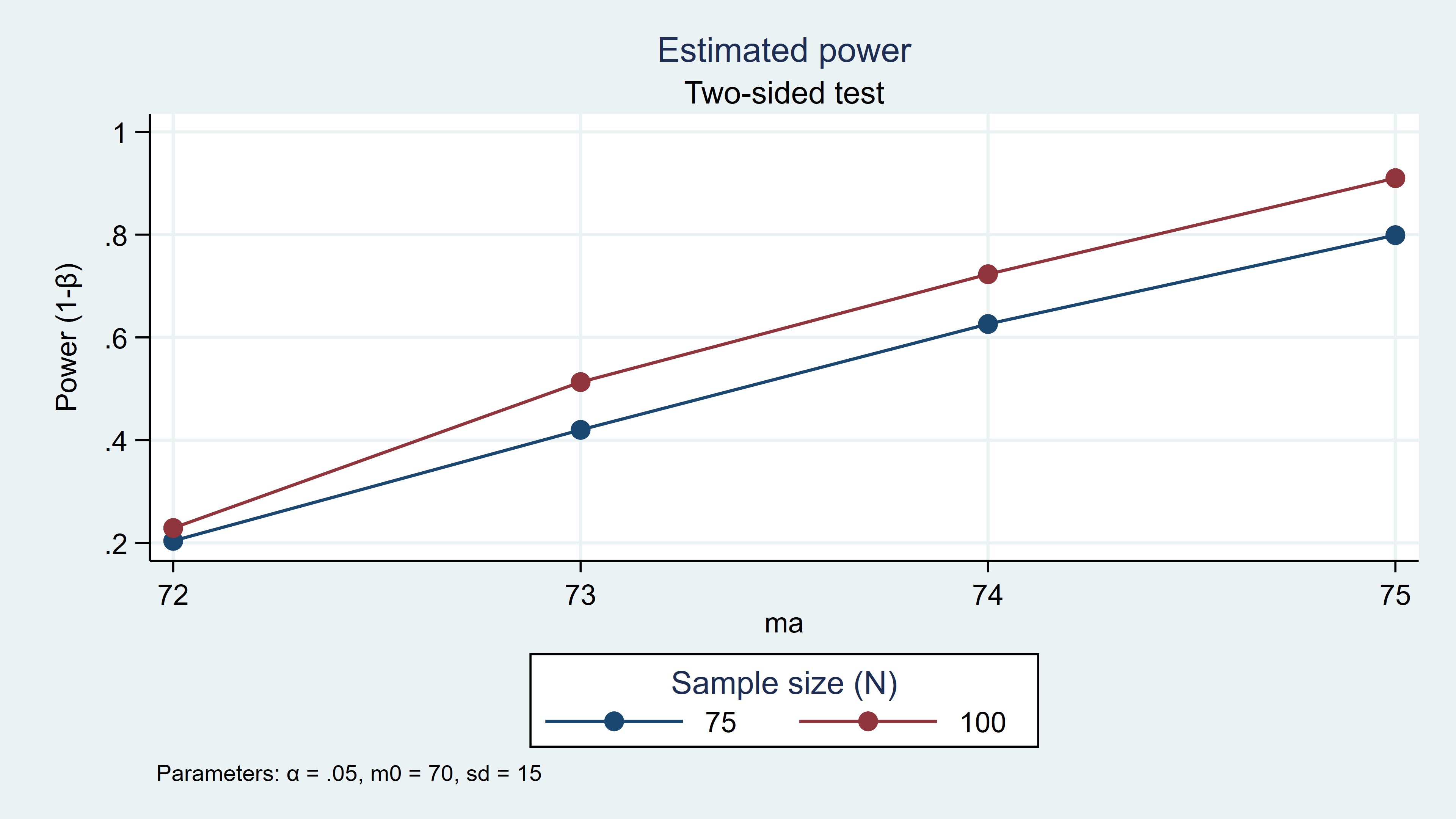
And you can plot the results of your power analysis by specifying xdimension in the graph option.
power simttest, n(75 100) m0(70) ma(72(1)75) sd(15) reps(1000) ///
   graph(xdimension(ma))
Figure 3: Simulated power for ma=72(1)75 given n=75 and n=100
So far I’ve shown you how to calculate power using Monte Carlo simulations and how to integrate those simulations into power. I started with a simple t test example so that we could focus on the programming and check our work with power onemean. Next time, I’ll show you how to write power commands to calculate power for linear and logistic regression models using Monte Carlo simulations. See [PSS] power usermethod for more information about adding your own methods to power.