An introduction to the lasso in Stata
Why is the lasso interesting?
The least absolute shrinkage and selection operator (lasso) estimates model coefficients and these estimates can be used to select which covariates should be included in a model. The lasso is used for outcome prediction and for inference about causal parameters. In this post, we provide an introduction to the lasso and discuss using the lasso for prediction. In the next post, we discuss using the lasso for inference about causal parameters.
The lasso is most useful when a few out of many potential covariates affect the outcome and it is important to include only the covariates that have an affect. “Few” and “many” are defined relative to the sample size. In the example discussed below, we observe the most recent health-inspection scores for 600 restaurants, and we have 100 covariates that could potentially affect each one’s score. We have too many potential covariates because we cannot reliably estimate 100 coefficients from 600 observations. We believe that only about 10 of the covariates are important, and we feel that 10 covariates are “a few” relative to 600 observations.
Given that only a few of the many covariates affect the outcome, the problem is now that we don’t know which covariates are important and which are not. The lasso produces estimates of the coefficients and solves this covariate-selection problem.
There are technical terms for our example situation. A model with more covariates than whose coefficients you could reliably estimate from the available sample size is known as a high-dimensional model. The assumption that the number of coefficients that are nonzero in the true model is small relative to the sample size is known as a sparsity assumption. More realistically, the approximate sparsity assumption requires that the number of nonzero coefficients in the model that best approximates the real world be small relative to the sample size.
In these technical terms, the lasso is most useful when estimating the coefficients in a high-dimensional, approximately sparse, model.
High-dimensional models are nearly ubiquitous in prediction problems and models that use flexible functional forms. In many cases, the many potential covariates are created from polynomials, splines, or other functions of the original covariates. In other cases, the many potential covariates come from administrative data, social media, or other sources that naturally produce huge numbers of potential covariates.
Predicting restaurant inspection scores
We use a series of examples to make our discussion of the lasso more accessible. These examples use some simulated data from the following problem. A health inspector in a small U.S. city wants to use social-media reviews to predict the health-inspection scores of restaurants. The inspector plans to add surprise inspections to the restaurants with the lowest-predicted health scores, using our predictions.
hsafety2.dta has 1 observation for each of 600 restaurants, and the score from the most recent inspection is in score. The percentage of a restaurant’s social-media reviews that contain a word like “dirty” could predict the inspection score. We identified 50 words, 30 word pairs, and 20 phrases whose occurrence percentages in reviews written in the three months prior to an inspection could predict the inspection score. The occurrence percentages of the 50 words are in word1 – word50. The occurrence percentages of 30-word pairs are in wpair1 – wpair30. The occurrence percentages of the 20 phrases are in phrase1 – phrase20.
Researchers widely use the following steps to find the best predictor.
- Divide the sample into training and validation subsamples.
- Use the training data to estimate the model parameters of each of the competing estimators.
- Use the validation data to estimate the out-of-sample mean squared error (MSE) of the predictions produced by each competing estimator.
- The best predictor is the estimator that produces the smallest out-of-sample MSE.
The ordinary least-squares (OLS) estimator is frequently included as a benchmark estimator when it is feasible. We begin the process with splitting the sample and computing the OLS estimates.
In the output below, we read the data into memory and use splitsample with the option split(.75 .25) to generate the variable sample, which is 1 for a 75% of the sample and 2 for the remaining 25% of the sample. The assignment of each observation in sample to 1 or 2 is random, but the rseed option makes the random assignment reproducible.
. use hsafety2

. splitsample , generate(sample) split(.75 .25) rseed(12345)

. label define slabel 1 "Training" 2 "Validation"

. label values sample slabel

. tabulate sample

     sample |      Freq.     Percent        Cum.
------------+-----------------------------------
   Training |        450       75.00       75.00
 Validation |        150       25.00      100.00
------------+-----------------------------------
      Total |        600      100.00
The one-way tabulation of sample produced by tabulate verifies that sample contains the requested 75%–25% division.
Next, we compute the OLS estimates using the data in the training sample and store the results in memory as ols.
. quietly regress score word1-word50 wpair1-wpair30 phrase1-phrase20
>         if sample==1

. estimates store ols
Now, we use lassogof with option over(sample) to compute the in-sample (Training) and out-of-sample (Validation) estimates of the MSE.
. lassogof ols, over(sample)

Penalized coefficients
-------------------------------------------------------------
Name             sample |         MSE    R-squared        Obs
------------------------+------------------------------------
ols                     |
               Training |    24.43515       0.5430        450
             Validation |    35.53149       0.2997        150
-------------------------------------------------------------
As expected, the estimated MSE is much smaller in the Training subsample than in the Validation sample. The out-of-sample estimate of the MSE is the more reliable estimator for the prediction error; see, for example, chapters 1, 2, and 3 in Hastie, Tibshirani, and Friedman (2009).
In this section, we introduce the lasso and compare its estimated out-of-sample MSE to the one produced by OLS.
What’s a lasso?
The lasso is an estimator of the coefficients in a model. What makes the lasso special is that some of the coefficient estimates are exactly zero, while others are not. The lasso selects covariates by excluding the covariates whose estimated coefficients are zero and by including the covariates whose estimates are not zero. There are no standard errors for the lasso estimates. The lasso’s ability to work as a covariate-selection method makes it a nonstandard estimator and prevents the estimation of standard errrors. In this post, we discuss how to use the lasso for inferential questions.
Tibshirani (1996) derived the lasso, and Hastie, Tibshirani, and Wainwright (2015) provide a textbook introduction.
The remainder of this section provides some details about the mechanics of how the lasso produces its coefficient estimates. There are different versions of the lasso for linear and nonlinear models. Versions of the lasso for linear models, logistic models, and Poisson models are available in Stata 16. We discuss only the lasso for the linear model, but the points we make generalize to the lasso for nonlinear models.
Like many estimators, the lasso for linear models solves an optimization problem. Specifically, the linear lasso point estimates \(\widehat{\boldsymbol{\beta}}\) are given by
$$
\widehat{\boldsymbol{\beta}} = \arg\min_{\boldsymbol{\beta}}
\left\{
\frac{1}{2n} \sum_{i=1}^n\left(y_i – {\bf x}_i\boldsymbol{\beta}’\right)^2
+\lambda\sum_{j=1}^p\omega_j\vert\beta_j\vert
\right\}
$$
where
- \(\lambda>0\) is the lasso penalty parameter,
- \(y\) is the outcome variable,
- \({\bf x}\) contains the \(p\) potential covariates,
- \(\boldsymbol{\beta}\) is the vector of coefficients on \({\bf x}\),
- \(\beta_j\) is the \(j\)th element of \(\boldsymbol{\beta}\),
- the \(\omega_j\) are parameter-level weights known as penalty loadings, and
- \(n\) is the sample size.
There are two terms in this optimization problem, the least-squares fit measure
$$\frac{1}{2n} \sum_{i=1}^n\left(y_i – {\bf x}_i\boldsymbol{\beta}’\right)^2$$
and the penalty term
$$\lambda\sum_{j=1}^p\omega_j\vert\boldsymbol{\beta}_j\vert$$
The parameters \(\lambda\) and the \(\omega_j\) are called “tuning” parameters. They specify the weight applied to the penalty term. When \(\lambda=0\), the linear lasso reduces to the OLS estimator. As \(\lambda\) increases, the magnitude of all the estimated coefficients is “shrunk” toward zero. This skrinkage occurs because the cost of each nonzero \(\widehat{\beta}_j\) increases with the penalty term that increases as \(\lambda\) increases.
The penalty term includes the absolute value of each \(\beta_j\). The absolute value function has a kink, sometimes called a check, at zero. The kink in the contribution of each coefficient to the penalty term causes some of the estimated coefficients to be exactly zero at the optimal solution. See section 2.2 of Hastie, Tibshirani, and Wainwright (2015) for more details.
There is a value \(\lambda_{\rm max}\) for which all the estimated coefficients are exactly zero. As \(\lambda\) decreases from \(\lambda_{\rm max}\), the number of nonzero coefficient estimates increases. For \(\lambda\in(0,\lambda_{\rm max})\), some of the estimated coefficients are exactly zero and some of them are not zero. When you use the lasso for covariate selection, covariates with estimated coefficients of zero are excluded, and covariates with estimated coefficients that are not zero are included.
That the number of potential covariates \(p\) can be greater than the sample size \(n\) is a much discussed advantage of the lasso. It is important to remember that the approximate sparsity assumption requires that the number of covariates that belong in the model (\(s\)) must be small relative to \(n\).
Selecting the lasso tuning parameters
The tuning parameters must be selected before using the lasso for prediction or model selection. The most frequent methods used to select the tuning parameters are cross-validation (CV), the adaptive lasso, and plug-in methods. In addition, \(\lambda\) is sometimes set by hand in a sensitivity analysis.
CV finds the \(\lambda\) that minimizes the out-of-sample MSE of the predictions. The mechanics of CV mimic the process using split samples to find the best out-of-sample predictor. The details are presented in an appendix.
CV is the default method of selecting the tuning parameters in the lasso command. In the output below, we use lasso to estimate the coefficients in the model for score, using the training sample. We specified the option rseed() to make our CV results reproducible.
. lasso linear score word1-word50 wpair1-wpair30 phrase1-phrase20
>         if sample==1, nolog rseed(12345)

Lasso linear model                          No. of obs        =        450
                                            No. of covariates =        100
Selection: Cross-validation                 No. of CV folds   =         10

--------------------------------------------------------------------------
         |                                No. of      Out-of-      CV mean
         |                               nonzero       sample   prediction
      ID |     Description      lambda     coef.    R-squared        error
---------+----------------------------------------------------------------
       1 |    first lambda    3.271123         0       0.0022       53.589
      25 |   lambda before    .3507518        22       0.3916     32.53111
    * 26 | selected lambda     .319592        25       0.3917     32.52679
      27 |    lambda after    .2912003        26       0.3914     32.53946
      30 |     last lambda    .2202824        30       0.3794     33.18254
--------------------------------------------------------------------------
* lambda selected by cross-validation.

. estimates store cv
We specified the option nolog to supress the CV log over the candidate values of \(\lambda\). The output reveals that CV selected a \(\lambda\) for which 25 of the 100 covariates have nonzero coefficients. We used estimates store to store these results under the name cv in memory.
We use cvplot to plot the CV function.
. cvplot, minmax
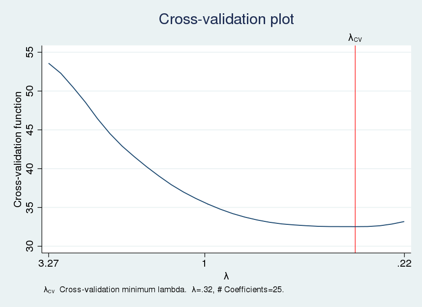
The CV function appears somewhat flat near the optimal \(\lambda\), which implies that nearby values of \(\lambda\) would produce similar out-of-sample MSEs.
The number of included covariates can vary substantially over the flat part of the CV function. We can investigate the variation in the number of selected covariates using a table called a lasso knot table. In the jargon of lasso, a knot is a value of \(\lambda\) for which a covariate is added or subtracted to the set of covariates with nonzero values. We use lassoknots to display the table of knots.
. lassoknots

-------------------------------------------------------------------------------------
       |              No. of   CV mean |
       |             nonzero     pred. |        Variables (A)dded, (R)emoved,
    ID |   lambda      coef.     error |             or left (U)nchanged
-------+-------------------------------+---------------------------------------------
     2 | 2.980526          2   52.2861 | A phrase3   phrase4
     3 | 2.715744          3  50.48463 | A phrase5
     4 | 2.474485          4  48.55981 | A word3
     6 | 2.054361          5  44.51782 | A phrase6
     9 | 1.554049          6  40.23385 | A wpair3
    10 | 1.415991          8  39.04494 | A wpair2    phrase2
    12 | 1.175581          9    36.983 | A word2
    14 | .9759878         10  35.42697 | A word31
    16 | .8102822         11   34.2115 | A word19
    17 |  .738299         12  33.75501 | A word4
    21 | .5088809         14  32.74808 | A word14    phrase7
    22 | .4636733         17  32.64679 | A word32    wpair19   wpair26
    23 | .4224818         19  32.56572 | A wpair15   wpair25
    24 | .3849497         22  32.53301 | A wpair24   phrase13  phrase14
  * 26 |  .319592         25  32.52679 | A word25    word30    phrase8
    27 | .2912003         26  32.53946 | A wpair11
    29 | .2417596         27  32.86193 | A wpair17
    30 | .2202824         30  33.18254 | A word23    word38    wpair4
-------------------------------------------------------------------------------------
* lambda selected by cross-validation.
The CV function is minimized at the \(\lambda\) with ID=26, and the lasso includes 25 covariates at this \(\lambda\) value. The flat part of the CV function includes the \(\lambda\) values with ID \(\in\{21,22,23,24,26,27\}\). Only 14 covariates are included by the lasso using the \(\lambda\) at ID=21. We will explore this observation using sensitivity analysis below.
CV tends to include extra covariates whose coefficients are zero in the model that best approximates the process that generated the data. This can affect the prediction performance of the CV-based lasso, and it can affect the performance of inferential methods that use a CV-based lasso for model selection. The adaptive lasso is a multistep version of CV. It was designed to exclude some of these extra covariates.
The first step of the adaptive lasso is CV. The second step does CV among the covariates selected in the first step. In this second step, the penalty loadings are \(\omega_j=1/| \widehat{\boldsymbol{\beta}}_j|\), where \(\widehat{\boldsymbol{\beta}}_j\) are the penalized estimates from the first step. Covariates with smaller-magnitude coefficients are more likely to be excluded in the second step. See Zou (2006) and Bühlmann and Van de Geer (2011) for more about the adaptive lasso and the tendency of the CV-based lasso to overselect. Also see Chetverikov, Liao, and Chernozhukov (2019) for formal results for the CV lasso and results that could explain this overselection tendency.
We specify the option selection(adaptive) below to cause lasso to use the adaptive lasso instead of CV to select the tuning parameters. We used estimates store to store the results under the name adaptive.
. lasso linear score word1-word50 wpair1-wpair30 phrase1-phrase20
>         if sample==1, nolog rseed(12345) selection(adaptive)

Lasso linear model                         No. of obs         =        450
                                           No. of covariates  =        100
Selection: Adaptive                        No. of lasso steps =          2

Final adaptive step results
--------------------------------------------------------------------------
         |                                No. of      Out-of-      CV mean
         |                               nonzero       sample   prediction
      ID |     Description      lambda     coef.    R-squared        error
---------+----------------------------------------------------------------
      31 |    first lambda    124.1879         0       0.0037     53.66569
      77 |   lambda before    1.719861        12       0.4238     30.81155
    * 78 | selected lambda    1.567073        12       0.4239      30.8054
      79 |    lambda after    1.427859        14       0.4237     30.81533
     128 |     last lambda    .0149585        22       0.4102     31.53511
--------------------------------------------------------------------------
* lambda selected by cross-validation in final adaptive step.

. estimates store adaptive
We see that the adaptive lasso included 12 instead of 25 covariates.
Plug-in methods tend to be even more parsimonious than the adaptive lasso. Plug-in methods find the value of the \(\lambda\) that is large enough to dominate the estimation noise. The plug-in method chooses \(\omega_j\) to normalize the scores of the (unpenalized) fit measure for each parameter. Given the normalized scores, it chooses a value for \(\lambda\) that is greater than the largest normalized score with a probability that is close to 1.
The plug-in-based lasso is much faster than the CV-based lasso and the adaptive lasso. In practice, the plug-in-based lasso tends to include the important covariates and it is really good at not including covariates that do not belong in the model that best approximates the data. The plug-in-based lasso has a risk of missing some covariates with large coefficients and finding only some covariates with small coefficients. See Belloni, Chernozhukov, and Wei (2016) and Belloni, et al. (2012) for details and formal results.
We specify the option selection(plugin) below to cause lasso to use the plug-in method to select the tuning parameters. We used estimates store to store the results under the name plugin.
. lasso linear score word1-word50 wpair1-wpair30 phrase1-phrase20
>         if sample==1, selection(plugin)

Computing plugin lambda ...
Iteration 1:     lambda = .1954567   no. of nonzero coef. =       8
Iteration 2:     lambda = .1954567   no. of nonzero coef. =       9
Iteration 3:     lambda = .1954567   no. of nonzero coef. =       9

Lasso linear model                          No. of obs        =        450
                                            No. of covariates =        100
Selection: Plugin heteroskedastic

--------------------------------------------------------------------------
         |                                No. of
         |                               nonzero    In-sample
      ID |     Description      lambda     coef.    R-squared          BIC
---------+----------------------------------------------------------------
     * 1 | selected lambda    .1954567         9       0.3524     2933.203
--------------------------------------------------------------------------
* lambda selected by plugin formula assuming heteroskedastic.

. estimates store plugin
The plug-in-based lasso included 9 of the 100 covariates, which is far fewer than included by the CV-based lasso or the adaptive lasso.
Comparing the predictors
We now have four different predictors for score: OLS, CV-based lasso, adaptive lasso, and plug-in-based lasso. The three lasso methods could predict score using the penalized coefficients estimated by lasso, or they could predict score using the unpenalized coefficients estimated by OLS, including only the covariates selected by lasso. The predictions that use the penalized lasso estimates are known as the lasso predictions and the predictions that use the unpenalized coefficients are known as the postselection predictions, or the postlasso predictions.
For linear models, Belloni and Chernozhukov (2013) present conditions in which the postselection predictions perform at least as well as the lasso predictions. Heuristically, one expects the lasso predictions from a CV-based lasso to perform better than the postselection predictions because CV chooses \(\lambda\) to make the best lasso predictions. Analogously, one expects the postselection predictions for the plug-in-based lasso to perform better than the lasso predictions because the plug-in tends to select a set of covariates close to those that best approximate the process that generated the data.
In practice, we estimate the out-of-sample MSE of the predictions for all estimators using both the lasso predictions and the postselection predictions. We select the one that produces the lowest out-of-sample MSE of the predictions.
In the output below, we use lassogof to compare the out-of-sample prediction performance of OLS and the lasso predictions from the three lasso methods.
. lassogof ols cv adaptive plugin if sample==2

Penalized coefficients
-------------------------------------------------
       Name |         MSE    R-squared        Obs
------------+------------------------------------
        ols |    35.53149       0.2997        150
         cv |    27.83779       0.4513        150
   adaptive |    27.83465       0.4514        150
     plugin |    32.29911       0.3634        150
-------------------------------------------------
For these data, the lasso predictions using the adaptive lasso performed a little bit better than the lasso predictions from the CV-based lasso.
In the output below, we compare the out-of-sample prediction performance of OLS and the lasso predictions from the three lasso methods using the postselection coefficient estimates.
. lassogof ols cv adaptive plugin if sample==2, postselection

Penalized coefficients
-------------------------------------------------
       Name |         MSE    R-squared        Obs
------------+------------------------------------
        ols |    35.53149       0.2997        150
         cv |    27.87639       0.4506        150
   adaptive |    27.79562       0.4522        150
     plugin |    26.50811       0.4775        150
-------------------------------------------------
It is not surprising that the plug-in-based lasso produces the smallest out-of-sample MSE. The plug-in method tends to select covariates whose postselection estimates do a good job of approximating the data.
The real competition tends to be between the lasso estimates from the best of the penalized lasso predictions and the postselection estimates from the plug-in-based lasso. In this case, the postselection estimates from the plug-in-based lasso produced the better out-of-sample predictions, and we would use these results to predict score.
The elastic net and ridge regression
The elastic net extends the lasso by using a more general penalty term. The elastic net was originally motivated as a method that would produce better predictions and model selection when the covariates were highly correlated. See Zou and Hastie (2005) for details.
The linear elastic net solves
$$
\widehat{\boldsymbol{\beta}} = \arg\min_{\boldsymbol{\beta}}
\left\{
\frac{1}{2n} \sum_{i=1}^n\left(y_i – {\bf x}_i\boldsymbol{\beta}’\right)^2
+\lambda\left[
\alpha\sum_{j=1}^p\vert\boldsymbol{\beta}_j\vert
+ \frac{(1-\alpha)}{2}
\sum_{j=1}^p\boldsymbol{\beta}_j^2
\right]
\right\}
$$
where \(\alpha\) is the elastic-net penalty parameter. Setting \(\alpha=0\) produces ridge regression. Setting \(\alpha=1\) produces lasso.
The elasticnet command selects \(\alpha\) and \(\lambda\) by CV. The option alpha() specifies the candidate values for \(\alpha\).
. elasticnet linear score word1-word50 wpair1-wpair30 phrase1-phrase20
>         if sample==1, alpha(.25 .5 .75) nolog rseed(12345)

Elastic net linear model                         No. of obs        =        450
                                                 No. of covariates =        100
Selection: Cross-validation                      No. of CV folds   =         10

-------------------------------------------------------------------------------
               |                               No. of      Out-of-      CV mean
               |                              nonzero       sample   prediction
alpha       ID |     Description      lambda    coef.    R-squared        error
---------------+---------------------------------------------------------------
0.750          |
             1 |    first lambda    13.08449        0       0.0062     53.79915
            39 |   lambda before    .4261227       24       0.3918     32.52101
          * 40 | selected lambda    .3882671       25       0.3922     32.49847
            41 |    lambda after    .3537745       27       0.3917     32.52821
            44 |     last lambda    .2676175       34       0.3788     33.21631
---------------+---------------------------------------------------------------
0.500          |
            45 |    first lambda    13.08449        0       0.0062     53.79915
            84 |     last lambda    .3882671       34       0.3823     33.02645
---------------+---------------------------------------------------------------
0.250          |
            85 |    first lambda    13.08449        0       0.0058     53.77755
           120 |     last lambda    .5633091       54       0.3759       33.373
-------------------------------------------------------------------------------
* alpha and lambda selected by cross-validation.

. estimates store enet
We see that the elastic net selected 25 of the 100 covariates.
For comparison, we also use elasticnet to perform ridge regression, with the penalty parameter selected by CV.
. elasticnet linear score word1-word50 wpair1-wpair30 phrase1-phrase20
>         if sample==1, alpha(0) nolog rseed(12345)

Elastic net linear model                         No. of obs        =        450
                                                 No. of covariates =        100
Selection: Cross-validation                      No. of CV folds   =         10

-------------------------------------------------------------------------------
               |                               No. of      Out-of-      CV mean
               |                              nonzero       sample   prediction
alpha       ID |     Description      lambda    coef.    R-squared        error
---------------+---------------------------------------------------------------
0.000          |
             1 |    first lambda    3271.123      100       0.0062     53.79914
            90 |   lambda before     .829349      100       0.3617     34.12734
          * 91 | selected lambda    .7556719      100       0.3621      34.1095
            92 |    lambda after    .6885401      100       0.3620     34.11367
           100 |     last lambda    .3271123      100       0.3480     34.86129
-------------------------------------------------------------------------------
* alpha and lambda selected by cross-validation.

. estimates store ridge
Ridge regression does not perform model selection and thus includes all the covariates.
We now compare the out-of-sample predictive ability of the CV-based lasso, the elastic net, ridge regression, and the plug-in-based lasso using the lasso predictions. (For elastic net and ridge regression, the “lasso predictions” are made using the coefficient estimates produced by the penalized estimator.)
. lassogof cv adaptive enet ridge plugin if sample==2

Penalized coefficients
-------------------------------------------------
       Name |         MSE    R-squared        Obs
------------+------------------------------------
         cv |    27.83779       0.4513        150
   adaptive |    27.83465       0.4514        150
       enet |    27.77314       0.4526        150
      ridge |    29.47745       0.4190        150
     plugin |    32.29911       0.3634        150
-------------------------------------------------
In this case, the penalized elastic-net coefficient estimates predict best out of sample among the lasso estimates. The postselection predictions produced by the plug-in-based lasso perform best overall. This can be seen by comparing the above output with the output below.
. lassogof cv adaptive enet plugin if sample==2, postselection

Penalized coefficients
-------------------------------------------------
       Name |         MSE    R-squared        Obs
------------+------------------------------------
         cv |    27.87639       0.4506        150
   adaptive |    27.79562       0.4522        150
       enet |    27.87639       0.4506        150
     plugin |    26.50811       0.4775        150
-------------------------------------------------
So we would use these postselection coefficient estimates from the plug-in-based lasso to predict score.
Sensitivity analysis
Sensitivity analysis is sometimes performed to see if a small change in the tuning parameters leads to a large change in the prediction performance. When looking at the output of lassoknots produced by the CV-based lasso, we noted that for a small increase in the CV function produced by the penalized estimates, there could be a significant reduction in the number of selected covariates. Restoring the cv estimates and repeating the lassoknots output, we see that
. estimates restore cv
(results cv are active now)

. lassoknots

-------------------------------------------------------------------------------------
       |              No. of   CV mean |
       |             nonzero     pred. |        Variables (A)dded, (R)emoved,
    ID |   lambda      coef.     error |             or left (U)nchanged
-------+-------------------------------+---------------------------------------------
     2 | 2.980526          2   52.2861 | A phrase3   phrase4
     3 | 2.715744          3  50.48463 | A phrase5
     4 | 2.474485          4  48.55981 | A word3
     6 | 2.054361          5  44.51782 | A phrase6
     9 | 1.554049          6  40.23385 | A wpair3
    10 | 1.415991          8  39.04494 | A wpair2    phrase2
    12 | 1.175581          9    36.983 | A word2
    14 | .9759878         10  35.42697 | A word31
    16 | .8102822         11   34.2115 | A word19
    17 |  .738299         12  33.75501 | A word4
    21 | .5088809         14  32.74808 | A word14    phrase7
    22 | .4636733         17  32.64679 | A word32    wpair19   wpair26
    23 | .4224818         19  32.56572 | A wpair15   wpair25
    24 | .3849497         22  32.53301 | A wpair24   phrase13  phrase14
  * 26 |  .319592         25  32.52679 | A word25    word30    phrase8
    27 | .2912003         26  32.53946 | A wpair11
    29 | .2417596         27  32.86193 | A wpair17
    30 | .2202824         30  33.18254 | A word23    word38    wpair4
-------------------------------------------------------------------------------------
* lambda selected by cross-validation.
lasso selected the \(\lambda\) with ID=26 and 25 covariates. We now use lassoselect to specify that the \(\lambda\) with ID=21 be the selected \(\lambda\) and store the results under the name hand.
. lassoselect id = 21
ID = 21  lambda = .5088809 selected

. estimates store hand
We now compute the out-of-sample MSE produced by the postselection estimates of the lasso whose \(\lambda\) has ID=21. The results are not wildly different and we would stick with those produced by the post-selection plug-in-based lasso.
. lassogof hand plugin if sample==2, postselection

Penalized coefficients
-------------------------------------------------
       Name |         MSE    R-squared        Obs
------------+------------------------------------
       hand |    27.71925       0.4537        150
     plugin |    26.50811       0.4775        150
-------------------------------------------------
Conclusion
This post has presented an introduction to the lasso and to the elastic net, and it has illustrated how to use them for prediction. There is much more information available in the Stata 16 LASSO manual. The next post will discuss using the lasso for inference about causal parameters.
References
Belloni, A., D. Chen, V. Chernozhukov, and C. Hansen. 2012. Sparse models and methods for optimal instruments with an application to eminent domain. Econometrica 80: 2369–2429.
Belloni, A., and V. Chernozhukov. 2013. Least squares after model selection in high-dimensional sparse models. Bernoulli 19: 521–547.
Belloni, A., V. Chernozhukov, and Y. Wei. 2016. Post-selection inference for generalized linear models with many controls. Journal of Business & Economic Statistics 34: 606–619.
Bühlmann, P., and S. Van de Geer. 2011. Statistics for High-Dimensional Data: Methods, Theory and Applications. Berlin: Springer.
Chetverikov, D., Z. Liao, and V. Chernozhukov. 2019. On cross-validated Lasso. arXiv Working Paper No. arXiv:1605.02214. http://arxiv.org/abs/1605.02214.
Hastie, T., R. Tibshirani, and J. Friedman. 2009. The Elements of Statistical Learning: Data Mining, Inference, and Prediction. 2nd ed. New York: Springer.
Hastie, T., R. Tibshirani, and M. Wainwright. 2015. Statistical Learning with Sparsity: The Lasso and Generalizations. Boca Rotaon, FL: CRC Press.
Tibshirani, R. 1996. Regression shrinkage and selection via the lasso. Journal of the Royal Statistical Society, Series B 58: 267–288.
Zou, H. 2006. The adaptive Lasso and its oracle properties. Journal of the American Statistical Association 101: 1418–1429.
Zou, H., and T. Hastie. 2005. Regularization and variable selection via the elastic net. Journal of the Royal Statistical Society, Series B 67: 301–320.
Appendix: K-fold cross-validation
Cross-validation finds the value for \(\lambda\) in a grid of candidate values \(\{\lambda_1, \lambda_2, \ldots, \lambda_Q\}\) that minimizes the MSE of the out-of-sample predictions. Cross-validation sets \(\omega_j=1\) or to user-specified values.
After you specify the grid, the sample is partitioned into \(K\) nonoverlapping subsets. For each grid value \(\lambda_q\), predict the out-of-sample squared errors using the following steps.
- For each \(k\in\{1,2,\ldots, K\}\),
- using the data not in partition \(k\), estimate the penalized coefficients \(\widehat{\boldsymbol{\beta}}\) with \(\lambda=\lambda_q\).
- using the data in partition \(k\), predict the out-of-sample squared errors.
The mean of these out-of-sample squared errors estimates the out-of-sample MSE of the predictions. The cross-validation function traces the values of these out-of-sample MSEs over the grid of candidate values for \(\lambda\). The \(\lambda_j\) that produces the smallest estimated out-of-sample MSE minimizes the cross-validation function, and it is selected.