Fun with frames
I have a confession. I wasn’t excited about the addition of frames to Stata 16. Yes, frames has been one of the most requested features for many years, and our website analytics show that frames is wildly popular. Adding frames was a smart decision and our customers are excited. But I have used Stata for over 20 years, and I have been perfectly happy using one dataset at a time. So I ignored frames.
Then I started working on an example for lasso using genetic data. I simulated patient data along with genetic data for each of 22 chromosomes saved in 22 separate datasets. Working with 23 datasets became cumbersome, so I thought I’d check out frames. I began by reading the manual and then tinkered with my genetic data. Along the way, I discovered a feature of frames that completely blew my mind. I’m going to show you that feature below, and I expect that it will blow your mind as well.
This blog post is not meant to be an introduction to frames. There is a detailed introduction to frames in the Stata 16 manual that will make you an expert. I simply want to show you some of the useful things that you can do with frames, including the following:
- Use multiple datasets simultaneously
- Frames and postestimation
- Linked frames and frval()
- Linked frames and frget
- Many frames
Use multiple datasets simultaneously
In this example, I have simulated patient data in one dataset and data from the NHANES study, which is a nationally representative sample of people in the United States. I would like to compare the results of regression models using my data with the results using the NHANES data. The NHANES data contain survey weights and my data do not. It might be possible to append the two datasets into a single dataset and use an indicator variable to differentiate between the observations from each study. But it would be difficult and frustrating to fit models with survey weights for some observations and not others. This is easy using frames.
Let’s begin by using frame create to create a new data frame named patients. Then, we can use the frame prefix to use the patient data in the data frame patients.
. frame create patients

. frame patients: use patients
We can then create another data frame named nhanes2 and webuse the dataset nhanes2.
. frame create nhanes2

. frame nhanes2: webuse nhanes2
We can type frame dir to verify that we have three data frames in memory. One is named default and the other two are the frames we created. We can also see the number of observations, the number of variables, and the datasets that are contained in each frame.
. frame dir
  default   0 x 0
  nhanes2   10351 x 58; nhanes2.dta
  patients  10000 x 41; patients.dta
Now, we can use the frames prefix to fit a linear regression model without survey weights using the patient data. And we can use the frames prefix to fit the same regression model with survey weights using the NHANES data. Note that I have used estimates store to store the parameter estimates in memory.
frame patients: regress sbp c.age##c.bmi
(output omitted)
estimates store patients
frame nhanes2: svy linearized : regress bpsystol c.age##c.bmi
(output omitted)
estimates store nhanes
Now, we can compare the results of our model fit to the two datasets using estimates table.
. estimates table patients nhanes

----------------------------------------
    Variable |  patients      nhanes
-------------+--------------------------
         age |   .5587357    .51511664
         bmi |   1.259132    1.2066527
             |
 c.age#c.bmi |  .00742543    .00200162
             |
       _cons |  70.882924     72.51606
----------------------------------------
Frames and postestimation
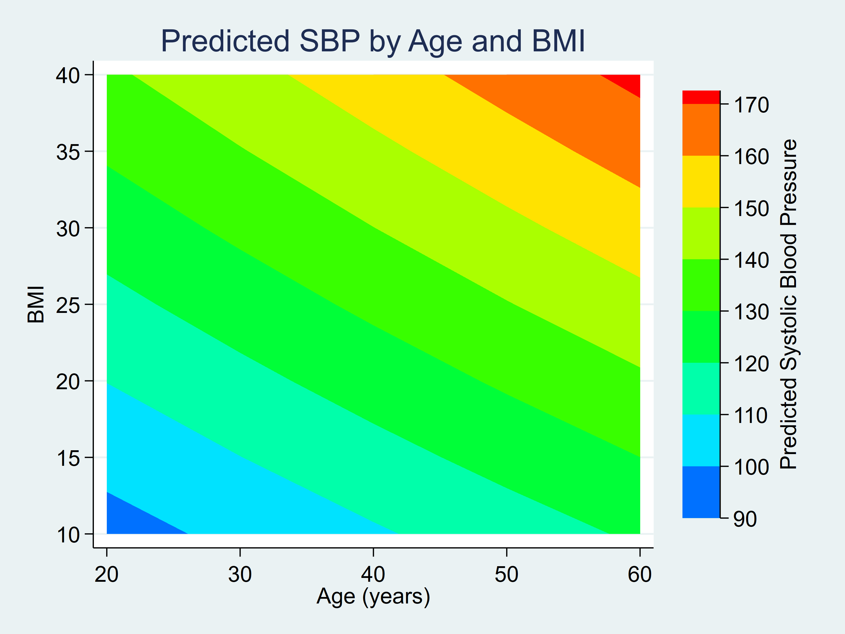
Next, we might wish to graph the predictions from the model using our patient data. We can do this using a technique that I describe in a Stata News article titled Visualizing continuous-by-continuous interactions with margins and twoway contour.
The basic strategy is to fit the model, use margins to estimate and save the predictions to a dataset, then use graph twoway contour to create the graph. In the Stata News article, I had to clear the main dataset to open the predictions dataset. Here we can simply create another frame to use the dataset that contains our predictions.
Let’s begin by using frame change so that we can run multiple commands using the patient data. Then we can fit our regression model and estimate the predictions using margins. Note that I have included the option saving(predictions, replace), which tells margins to store the predictions to a dataset named predictions.
. frame change patients

. regress sbp c.age##c.bmi

      Source |       SS           df       MS      Number of obs   =    10,000
-------------+----------------------------------   F(3, 9996)      =  14015.35
       Model |   1670892.7         3  556964.234   Prob > F        =    0.0000
    Residual |  397237.042     9,996  39.7396001   R-squared       =    0.8079
-------------+----------------------------------   Adj R-squared   =    0.8079
       Total |  2068129.74     9,999  206.833658   Root MSE        =    6.3039

------------------------------------------------------------------------------
         sbp |      Coef.   Std. Err.      t    P>|t|     [95% Conf. Interval]
-------------+----------------------------------------------------------------
         age |   .5587357   .0865853     6.45   0.000     .3890112    .7284602
         bmi |   1.259132   .1758975     7.16   0.000     .9143375    1.603927
             |
 c.age#c.bmi |   .0074254   .0034766     2.14   0.033     .0006105    .0142404
             |
       _cons |   70.88292   4.305602    16.46   0.000     62.44308    79.32277
------------------------------------------------------------------------------

. margins, at(age=(20(10)60) bmi=(10(5)40)) saving(predictions, replace)
(Output omitted)
Now, we can create a new frame named contour, change to that frame, and use the dataset predictions.
. frame create contour

. frame change contour

. use predictions
(Created by command margins; also see char list)
The variable _at1 in the predictions dataset contains age, _at2 contains BMI, and _margin contains the linear predictions.
. describe _at1 _at2 _margin

              storage   display    value
variable name   type    format     label      variable label
------------------------------------------------------------------------
_at1            byte    %9.0g                 age in years
_at2            byte    %9.0f                 Body Mass Index (BMI)
_margin         float   %9.0g                 Linear prediction, predict()

. list _at1 _at2 _margin in 1/5

     +------------------------+
     | _at1   _at2    _margin |
     |------------------------|
  1. |   20     10   96.13405 |
  2. |   20     15   103.1722 |
  3. |   20     20   110.2104 |
  4. |   20     25   117.2487 |
  5. |   20     30   124.2869 |
     +------------------------+
We can rename those variables and create a contour plot of the predictions.
. rename _at1 age

. rename _at2 bmi

. rename _margin pr_sbp

. twoway (contour pr_sbp bmi age, ccuts(90(10)170)),            ///
>         xlabel(20(10)60)  ylabel(10(5)40, angle(horizontal))  ///
>         xtitle("Age (years)") ytitle("BMI")                   ///
>         ztitle("Predicted Systolic Blood Pressure")           ///
>         title("Predicted SBP by Age and BMI")
Figure 1: Contour Plot for Predicted SBP by Age and BMI
Linked frames and frval()
We can also link two frames together using frlink. Let’s open another dataset named hospital in a new frame named hospital.
. frame create hospital

. frame change hospital

. use hospital

. list in 1/5, abbrev(10)

     +----------------------+
     | hospitalid   avgcost |
     |----------------------|
  1. |          1   135,242 |
  2. |          2   135,372 |
  3. |          3   134,467 |
  4. |          4   132,953 |
  5. |          5   134,622 |
     +----------------------+
The hospital dataset contains the variable hospitalid and a variable named avgcost, which is the average cost of heart bypass surgery at each hospital.
The patients dataset contains a variable named payment, which is the amount that each patient paid for heart bypass surgery. The variable hospitalid tells us the hospital at which each patient had surgery.
. frame change patients

. list patientid hospitalid payment in 1/5, abbrev(10)

     +----------------------------------+
     | patientid   hospitalid   payment |
     |----------------------------------|
  1. |         1           10   121,255 |
  2. |         2           18    90,164 |
  3. |         3            5   156,731 |
  4. |         4            6    98,256 |
  5. |         5           13   140,604 |
     +----------------------------------+
We can link the patient frame with the hospital frame using frlink. Each value of hospitalid appears many times in the patients frame and only once in the hospital frame. We can specify a “many-to-one” link by typing frlink m:1. And frame(hospital) tells frlink to link the current frame (patients) with the hospital frame.
. frlink m:1 hospitalid, frame(hospital)
  (all observations in frame patients matched)
Now that our frames are linked, we can use frval() to access values of variables in frames outside the current frame. For example, we might wish to calculate how much a patient paid for heart bypass surgery relative to the average cost at the hospital where the surgery was performed. We can generate a new variable named rel_payment, which is equal to the ratio of payment in the current frame (patients), divided by avgcost in the hospital frame. The function frval(hospital, avgcost) accesses the value of avgcost in the hospital frame.
. generate rel_payment = payment / frval(hospital, avgcost)

. list patientid hospitalid payment rel_payment in 1/5, abbrev(16)

     +------------------------------------------------+
     | patientid   hospitalid   payment   rel_payment |
     |------------------------------------------------|
  1. |         1           10   121,255      .8999608 |
  2. |         2           18    90,164      .6621906 |
  3. |         3            5   156,731      1.164228 |
  4. |         4            6    98,256      .7454461 |
  5. |         5           13   140,604      1.033123 |
     +------------------------------------------------+
Patient 3 in the list above paid $156,731 for surgery at Hospital 5. The hospital data above show that the average cost of the surgery at Hospital 5 was $134,622. The value of rel_payment tells us that patient 3 paid 16% more for their surgery than the average cost at hospital 5.
Linked frames and frget
We can also copy variables from one linked frame to another frame using frget. In this example, we have another dataset named longitudinal, which contains repeated observations of bmi and sbp over five years. Let’s create a new data frame named long for this dataset.
. frame create long

. frame change long

. use longitudinal

. list in 1/10, abbrev(10)

     +-----------------------------+
     | patientid   age   bmi   sbp |
     |-----------------------------|
  1. |         1    44    25   139 |
  2. |         1    45    26   144 |
  3. |         1    46    27   147 |
  4. |         1    47    25   137 |
  5. |         1    48    25   139 |
     |-----------------------------|
  6. |         2    69    26   164 |
  7. |         2    70    25   166 |
  8. |         2    71    28   169 |
  9. |         2    72    27   171 |
 10. |         2    73    24   165 |
     +-----------------------------+
We would like to fit a multilevel model for these longitudinal data stored in the long frame, adjusting for the effects of sex and race, which are stored in the patients frame. Let’s begin by using frlink to link the two frames.
. frlink m:1 patientid, frame(patients)
  (all observations in frame long matched)
Next, we can use frget to copy the variables sex and race from the patients frame to the current frame (long).
. frget sex race, from(patients)
  (2 variables copied from linked frame)

. list in 1/10, abbrev(10)

     +---------------------------------------------------------+
     | patientid   age   bmi   sbp   patients      sex    race |
     |---------------------------------------------------------|
  1. |         1    44    25   139          1     Male   White |
  2. |         1    45    26   144          1     Male   White |
  3. |         1    46    27   147          1     Male   White |
  4. |         1    47    25   137          1     Male   White |
  5. |         1    48    25   139          1     Male   White |
     |---------------------------------------------------------|
  6. |         2    69    26   164          2   Female   White |
  7. |         2    70    25   166          2   Female   White |
  8. |         2    71    28   169          2   Female   White |
  9. |         2    72    27   171          2   Female   White |
 10. |         2    73    24   165          2   Female   White |
     +---------------------------------------------------------+
Now, we can fit our multilevel model.
. mixed sbp i.sex i.race c.age##c.bmi || patientid:, nolog noheader

------------------------------------------------------------------------------
         sbp |      Coef.   Std. Err.      z    P>|z|     [95% Conf. Interval]
-------------+----------------------------------------------------------------
         sex |
     Female  |   .1787433   .1213193     1.47   0.141    -.0590382    .4165247
             |
        race |
      Black  |   .0270491   .1957962     0.14   0.890    -.3567045    .4108026
      Other  |   .0539184   .4375286     0.12   0.902    -.8036219    .9114587
             |
         age |     .48519   .0158596    30.59   0.000     .4541058    .5162742
         bmi |   1.175005   .0322024    36.49   0.000     1.111889     1.23812
             |
 c.age#c.bmi |    .010324   .0006217    16.61   0.000     .0091055    .0115424
             |
       _cons |    72.9325   .8130494    89.70   0.000     71.33895    74.52605
------------------------------------------------------------------------------

------------------------------------------------------------------------------
  Random-effects Parameters  |   Estimate   Std. Err.     [95% Conf. Interval]
-----------------------------+------------------------------------------------
patientid: Identity          |
                  var(_cons) |    35.8953   .5189054      34.89254    36.92689
-----------------------------+------------------------------------------------
               var(Residual) |   3.973389   .0280961      3.918702     4.02884
------------------------------------------------------------------------------
LR test vs. linear model: chibar2(01) = 76974.75      Prob >= chibar2 = 0.0000
Many frames
I mentioned earlier that I’ve been experimenting with simulated genetic data and lasso. Let’s assume that I sent blood samples from 500 patients to a lab and they sent us 22 datasets. Each of the 22 datasets contains indicator variables for the presence of a particular genetic marker. Let’s take a look at the files.
. ls

  79.6M   7/22/19  9:40  chromosome1.dta
  42.8M   7/22/19  9:40  chromosome10.dta
  43.2M   7/22/19  9:40  chromosome11.dta
  42.6M   7/22/19  9:40  chromosome12.dta
  36.6M   7/22/19  9:40  chromosome13.dta
  34.2M   7/22/19  9:40  chromosome14.dta
  32.6M   7/22/19  9:40  chromosome15.dta
  28.8M   7/22/19  9:40  chromosome16.dta
  26.6M   7/22/19  9:40  chromosome17.dta
  25.7M   7/22/19  9:40  chromosome18.dta
  18.7M   7/22/19  9:40  chromosome19.dta
  77.4M   7/22/19  9:40  chromosome2.dta
  20.6M   7/22/19  9:40  chromosome20.dta
  14.9M   7/22/19  9:40  chromosome21.dta
  16.2M   7/22/19  9:40  chromosome22.dta
  63.4M   7/22/19  9:40  chromosome3.dta
  60.8M   7/22/19  9:40  chromosome4.dta
  58.0M   7/22/19  9:40  chromosome5.dta
  54.6M   7/22/19  9:40  chromosome6.dta
  51.0M   7/22/19  9:40  chromosome7.dta
  46.4M   7/22/19  9:40  chromosome8.dta
  44.3M   7/22/19  9:41  chromosome9.dta
The first thing that I notice is that each file is fairly large. The file chromosome1.dta is 79.6 megabytes. Let’s describe the contents of the file chromosome1.dta without opening the file.
. describe using chromosome1, short

Contains data
  obs:           500                          15 Jul 2019 17:30
 vars:        73,090
Sorted by:
This dataset contains 500 observations on 73,090 variables, which tells me that I will need to use Stata/MP to open this file. Stata/MP can open files with up to 120,000 variables and over 20 billion observations. All the examples below require Stata/MP.
We will also need to change some of Stata’s defaults to work with these large datasets.
. set segmentsize 100m    // Default is 32m

. set maxvar 80000       // Default is 5000
set segmentsize allocates memory for data in units of segmentsize. Smaller values of segmentsize can result in more efficient use of available memory but require Stata to jump around more. Our largest file is chromosome1.dta, which is 79.6 megabytes, so I have changed the segmentsize to 100 megabytes.
set maxvar changes the maximum number of variables allowed from the default of 5,000 to 80,000.
You can read more about the details of memory management in the manual.
Now we are ready to open the dataset chromosome1.dta.
. frame create chr1

. frame change chr1

. use chromosome1

. list id gene1_snp1 gene1_snp2 gene1_snp3 gene1_snp4 gene1_snp5 in 1/5, abbrev(12)

     +---------------------------------------------------------------------+
     | id   gene1_snp1   gene1_snp2   gene1_snp3   gene1_snp4   gene1_snp5 |
     |---------------------------------------------------------------------|
  1. |  1            0            0            0            1            0 |
  2. |  2            0            0            0            0            0 |
  3. |  3            0            0            0            0            0 |
  4. |  4            1            0            0            1            1 |
  5. |  5            0            0            0            1            0 |
     +---------------------------------------------------------------------+
The list above includes only 6 of the 73,090 variables in the dataset. The variable id in the long frame corresponds to the variable patientid in the patients frame. So we will need to rename the variable patientid to id before we can link the two frames.
. frame patients: rename patientid id

. frlink 1:1 id, frame(patients)
  (all observations in frame chr1 matched)
Next, we can use frget to copy the variables sbp, age, sex, race, and bmi from the patients frame to the current frame (chr1).
. frget sbp age sex race bmi, from(patients)
  (5 variables copied from linked frame)
Now, we’re ready to use dsregress to fit an inferential lasso model that includes the dependent variable sbp, variables of interest age, sex, race, and bmi, and controlling for the 73,089 genetic variables.
. dsregress sbp i.sex i.race c.age##c.bmi, controls(gene*) rseed(16)

Estimating lasso for sbp using plugin

(notes omitted)

Double-selection linear model         Number of obs               =        500
                                      Number of controls          =     73,089
                                      Number of selected controls =          1
                                      Wald chi2(6)                =    2214.13
                                      Prob > chi2                 =     0.0000

------------------------------------------------------------------------------
             |               Robust
         sbp |      Coef.   Std. Err.      z    P>|z|     [95% Conf. Interval]
-------------+----------------------------------------------------------------
         sex |
     Female  |    .509223   .5573234     0.91   0.361    -.5831107    1.601557
             |
        race |
      Black  |  -.5006748   .6594229    -0.76   0.448     -1.79312    .7917703
      Other  |   .1005796   .7350127     0.14   0.891    -1.340019    1.541178
             |
         age |  -.2644798   .3941441    -0.67   0.502    -1.036988    .5080285
         bmi |  -.5820806    .806618    -0.72   0.471    -2.163023    .9988617
             |
 c.age#c.bmi |   .0416917   .0158851     2.62   0.009     .0105574     .072826
------------------------------------------------------------------------------
Note: Chi-squared test is a Wald test of the coefficients of the variables
      of interest jointly equal to zero. Lassos select controls for model
      estimation. Type lassoinfo to see number of selected variables in each
      lasso.
We just fit a model that includes over 70,000 variables!
I told you at the beginning that I discovered a feature of frames that blew my mind, and you may be guessing that was it. But it wasn’t.
Stata/MP can open datasets with up to 120,000 variables and over 20 billion observations. While I was experimenting with my genetics examples, I wondered “Is it 120,000 variables total or 120,000 variables in each frame?” So I created one frame for chromosome 1 with 73,090 variables and another frame for chromosome 2 with 71,101. That’s 144,191 variables in memory at one time! So I got carried away and wrote the following loop:
forvalues i = 1/22 {

   frame create chr`i'

   frame change chr`i'

   use chromosome`i'

   frlink 1:1 id, frame(patients)

   frget sbp age sex race bmi, from(patients)

}
I had over 900,000 variables open in Stata simultaneously! This blew my mind. Perhaps it blows your mind too. If it doesn’t, consider that Stata/MP can use up to 100 frames simultaneously. Which means that Stata/MP can theoretically use 12,000,000 variables! That’s a lot of data. And that’s some of what you can do with frames in Stata 16.