COVID-19 time-series data from Johns Hopkins University
In my last post, we learned how to import the raw COVID-19 data from the Johns Hopkins GitHub repository. This post will demonstrate how to convert the raw data to time-series data. We’ll also create some tables and graphs along the way.
Let’s look at the raw COVID-19 data that we saved earlier.
. use covid19_raw, clear

. describe

Contains data from covid19_raw.dta
  obs:        11,341
 vars:            12                          24 Mar 2020 12:55
------------------------------------------------------------------------
              storage   display    value
variable name   type    format     label      variable label
------------------------------------------------------------------------
provincestate   str43   %43s                  Province/State
countryregion   str32   %32s                  Country/Region
lastupdate      str19   %19s                  Last Update
confirmed       long    %8.0g                 Confirmed
deaths          int     %8.0g                 Deaths
recovered       long    %8.0g                 Recovered
latitude        float   %9.0g                 Latitude
longitude       float   %9.0g                 Longitude
fips            long    %12.0g                FIPS
admin2          str21   %21s                  Admin2
active          long    %12.0g                Active
combined_key    str44   %44s                  Combined_Key
------------------------------------------------------------------------
Sorted by:
Our dataset contains 11,341 observations on 12 variables. Let’s list the first five observations for lastupdate.
. list lastupdate in 1/5

     +-----------------+
     |      lastupdate |
     |-----------------|
  1. | 1/22/2020 17:00 |
  2. | 1/22/2020 17:00 |
  3. | 1/22/2020 17:00 |
  4. | 1/22/2020 17:00 |
  5. | 1/22/2020 17:00 |
     +-----------------+
lastupdate is the update time and date for each observation in the dataset. The data include the date followed by a space followed by time.
Let’s also look at the last five observations in the dataset.
. list lastupdate in -5/l

       +---------------------+
       |          lastupdate |
       |---------------------|
11337. | 2020-03-23 23:19:21 |
11338. | 2020-03-23 23:19:21 |
11339. | 2020-03-23 23:19:21 |
11340. | 2020-03-23 23:19:21 |
11341. | 2020-03-23 23:19:21 |
       +---------------------+
The last five observations contain similar information but in a different format. Unfortunately, the data for lastupdate were not stored consistently in the raw data files. We could examine the different ways dates were saved in lastupdate across the different files and develop a strategy to extract the dates. But we know the date for each file because it is part of the name for each raw data file. In my previous posts, we created a consistently formatted date when we imported the raw data. A simple solution would be to save that date as a variable when we import the raw data files. Let’s generate a variable named tempdate in each raw data file.
local URL = "https://raw.githubusercontent.com/CSSEGISandData/COVID-19/master/csse_covid_19_data/csse_covid_19_daily_reports/"

forvalues month = 1/12 {

   forvalues day = 1/31 {

      local month = string(`month', "%02.0f")

      local day = string(`day', "%02.0f")

      local year = "2020"

      local today = "`month'-`day'-`year'"

      local FileName = "`URL'`today'.csv"

      clear

      capture import delimited "`FileName'"

      capture confirm variable ïprovincestate

      if _rc == 0 {

         rename ïprovincestate provincestate

         label variable provincestate "Province/State"

      }

      capture rename province_state provincestate

      capture rename country_region countryregion

      capture rename last_update lastupdate

      capture rename lat latitude

      capture rename long longitude

      generate tempdate = "`today'"

      capture save "`today'", replace

   }

}

clear

forvalues month = 1/12 {

   forvalues day = 1/31 {

      local month = string(`month', "%02.0f")

      local day = string(`day', "%02.0f")

      local year = "2020"

      local today = "`month'-`day'-`year'"

      capture append using "`today'"

   }

}
We can check our work by listing the observations. Below, I have listed the first five observations and the last five observations in our combined raw dataset.
. list tempdate in 1/5

     +------------+
     |   tempdate |
     |------------|
  1. | 01-22-2020 |
  2. | 01-22-2020 |
  3. | 01-22-2020 |
  4. | 01-22-2020 |
  5. | 01-22-2020 |
     +------------+

. list tempdate in -5/l

       +------------+
       |   tempdate |
       |------------|
11337. | 03-23-2020 |
11338. | 03-23-2020 |
11339. | 03-23-2020 |
11340. | 03-23-2020 |
11341. | 03-23-2020 |
       +------------+
The date data saved in tempdate are stored consistently, but the data are still stored as a string. We can use the date() function to convert tempdate to a number. The date(s1,s2) function returns a number based on two arguments, s1 and s2. The argument s1 is the string we wish to act upon and the argument s2 is the order of the day, month, and year in s1. Our tempdate variable is stored with the month first, the day second, and the year third. So we can type s2 as MDY, which indicates that Month is followed by Day, which is followed by Year. We can use the date() function below to convert the string date 03-23-2020 to a number.
. display date("03-23-2020", "MDY")
21997
The date() function returned the number 21997. That doesn’t look like a date to you and me, but it indicates the number of days since January 1, 1960. The example below shows that 01-01-1960 is the 0 for our time data.
. display date("01-01-1960", "MDY")
0
We can change the way the number is displayed by applying a date format to the number.
. display %tdNN/DD/CCYY date("03-23-2020", "MDY")
03/23/2020
Let’s use date() to generate a new variable named date.
. generate date = date(tempdate, "MDY")

. list lastupdate tempdate date in -5/l

       +------------------------------------------+
       |          lastupdate     tempdate    date |
       |------------------------------------------|
11337. | 2020-03-23 23:19:21   03-23-2020   21997 |
11338. | 2020-03-23 23:19:21   03-23-2020   21997 |
11339. | 2020-03-23 23:19:21   03-23-2020   21997 |
11340. | 2020-03-23 23:19:21   03-23-2020   21997 |
11341. | 2020-03-23 23:19:21   03-23-2020   21997 |
       +------------------------------------------+
Next, we can use format to display the numbers in date in a way that looks familiar to you and me.
. format date %tdNN/DD/CCYY

. list lastupdate tempdate date in -5/l

       +-----------------------------------------------+
       |          lastupdate     tempdate         date |
       |-----------------------------------------------|
11337. | 2020-03-23 23:19:21   03-23-2020   03/23/2020 |
11338. | 2020-03-23 23:19:21   03-23-2020   03/23/2020 |
11339. | 2020-03-23 23:19:21   03-23-2020   03/23/2020 |
11340. | 2020-03-23 23:19:21   03-23-2020   03/23/2020 |
11341. | 2020-03-23 23:19:21   03-23-2020   03/23/2020 |
       +-----------------------------------------------+
Now, we have a date variable in our dataset that can be used with Stata’s time-series features and for other calculations.
Let’s save this dataset so that we don’t have to download the raw data for each of the following examples.
. save covid19_date, replace
file covid19_date.dta saved
Create time-series data
Let’s keep the data for the United States and list the data for January 26, 2020.
. keep if countryregion=="US"
(6,545 observations deleted)

. list date confirmed deaths recovered           ///
      if date==date("1/26/2020", "MDY"), abbreviate(13)

      +---------------------------------------------+
      |       date   confirmed   deaths   recovered |
      |---------------------------------------------|
   7. | 01/26/2020           1        .           . |
   8. | 01/26/2020           1        .           . |
   9. | 01/26/2020           2        .           . |
  10. | 01/26/2020           1        .           . |
      +---------------------------------------------+
There were four observations for the United States on January 26, 2020, and five confirmed cases of COVID-19. We would like our time-series data to contain all five confirmed cases in a single observation for a single date. We can use collapse to aggregate the data by date.
. collapse (sum) confirmed deaths recovered, by(date)

. list date confirmed deaths recovered           ///
      if date==date("1/26/2020", "MDY"), abbreviate(13)

     +---------------------------------------------+
     |       date   confirmed   deaths   recovered |
     |---------------------------------------------|
  5. | 01/26/2020           5        0           0 |
     +---------------------------------------------+
Let’s use the data for all countries and collapse the dataset by date.
. use covid19_date, clear

. collapse (sum) confirmed deaths recovered, by(date)
We can describe our new dataset and see that it contains the variables date, confirmed, deaths, and recovered. The variable labels tell us that confirmed, deaths, and recovered are the sum of each variable for each value of date.
. describe

Contains data
  obs:            60
 vars:             4
------------------------------------------------------------------------
              storage   display    value
variable name   type    format     label      variable label
------------------------------------------------------------------------
date            float   %td..
confirmed       double  %8.0g                 (sum) confirmed
deaths          double  %8.0g                 (sum) deaths
recovered       double  %8.0g                 (sum) recovered
------------------------------------------------------------------------
Sorted by: date
     Note: Dataset has changed since last saved.
We can list the first five observations to verify that we have one value of each variable for each date.
. list in 1/5, abbreviate(9)

     +---------------------------------------------+
     |       date   confirmed   deaths   recovered |
     |---------------------------------------------|
  1. | 01/22/2020         555       17          28 |
  2. | 01/23/2020         653       18          30 |
  3. | 01/24/2020         941       26          36 |
  4. | 01/25/2020        1438       42          39 |
  5. | 01/26/2020        2118       56          52 |
     +---------------------------------------------+
The counts are large and will likely grow larger. We can make our data easier to read by using format to add commas.
. format %8.0fc confirmed deaths recovered

. list, abbreviate(9)

     +---------------------------------------------+
     |       date   confirmed   deaths   recovered |
     |---------------------------------------------|
  1. | 01/22/2020         555       17          28 |
  2. | 01/23/2020         653       18          30 |
  3. | 01/24/2020         941       26          36 |
  4. | 01/25/2020       1,438       42          39 |
  5. | 01/26/2020       2,118       56          52 |
     |---------------------------------------------|
  6. | 01/27/2020       2,927       82          61 |

                     (Output omitted)

 58. | 03/19/2020     242,713    9,867      84,962 |
 59. | 03/20/2020     272,167   11,299      87,403 |
 60. | 03/21/2020     304,528   12,973      91,676 |
     |---------------------------------------------|
 61. | 03/22/2020     335,957   14,634      97,882 |
 62. | 03/23/2020     378,287   16,497     100,958 |
     +---------------------------------------------+
Now, we can use tsset to specify the structure of our time-series data, which will allow us to use Stata’s time-series features.
. tsset date, daily
        time variable:  date, 01/22/2020 to 03/23/2020
                delta:  1 day
Next, I would like to calculate the number of new cases reported each day. This is easy using time-series operators. The time-series operator D.varname calculates the difference between an observation and the preceding observation in varname. Let’s consider the value of confirmed for observation 2, which is 653. The preceding value of confirmed, observation 1, is 555. So D.confirmed for observation 2 is 653 – 555, which equals 98. The data for newcases in observation 1 are missing because there are no data preceding observation 1.
. generate newcases = D.confirmed
(1 missing value generated)

. list, abbreviate(9)

     +--------------------------------------------------------+
     |       date   confirmed   deaths   recovered   newcases |
     |--------------------------------------------------------|
  1. | 01/22/2020         555       17          28          . |
  2. | 01/23/2020         653       18          30         98 |
  3. | 01/24/2020         941       26          36        288 |
  4. | 01/25/2020       1,438       42          39        497 |
  5. | 01/26/2020       2,118       56          52        680 |
     |--------------------------------------------------------|
  6. | 01/27/2020       2,927       82          61        809 |

                         (Output omitted)

 58. | 03/19/2020     242,713    9,867      84,962      27798 |
 59. | 03/20/2020     272,167   11,299      87,403      29454 |
 60. | 03/21/2020     304,528   12,973      91,676      32361 |
     |--------------------------------------------------------|
 61. | 03/22/2020     335,957   14,634      97,882      31429 |
 62. | 03/23/2020     378,287   16,497     100,958      42330 |
     +--------------------------------------------------------+
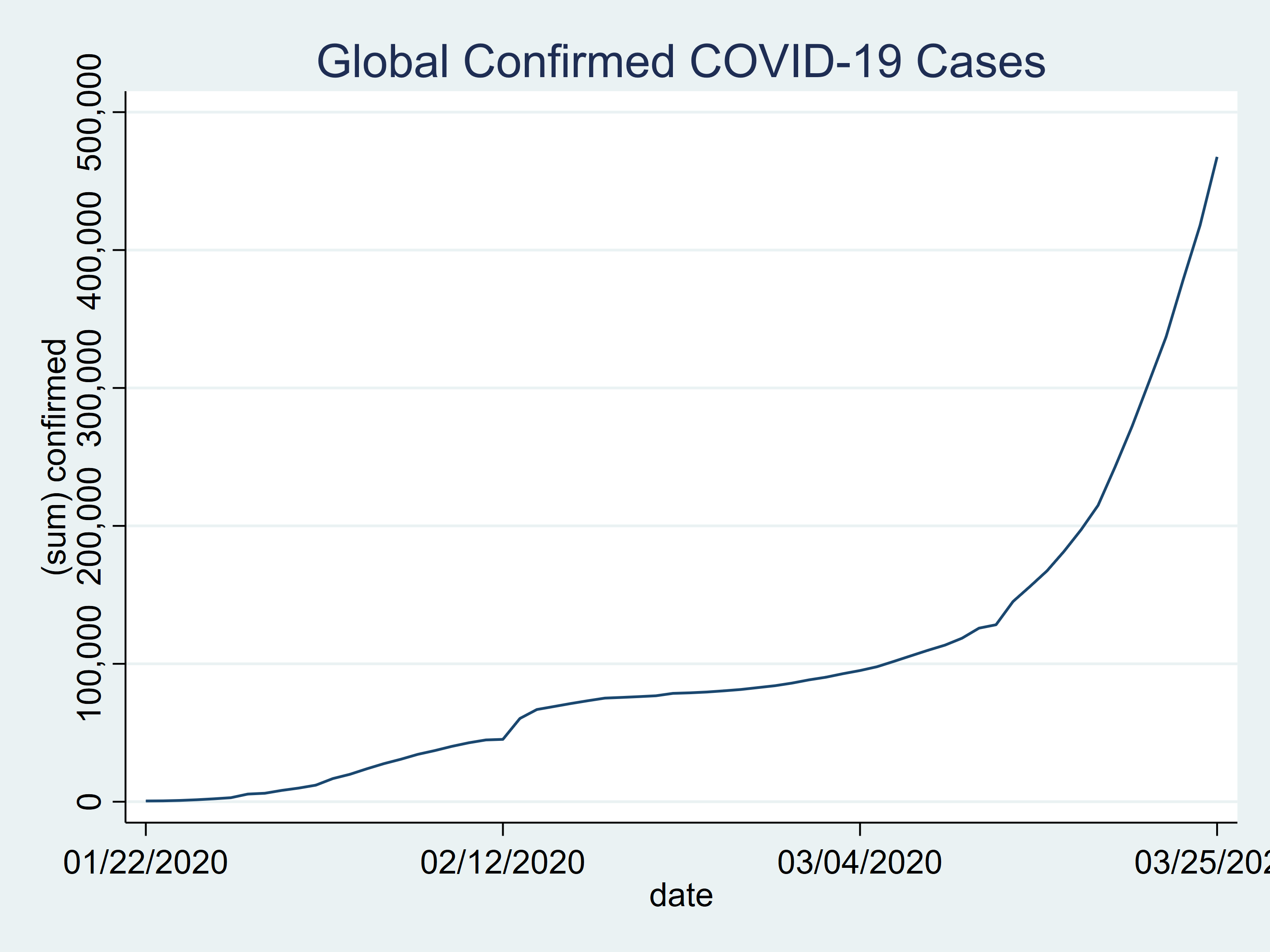
Let’s create a time-series plot for the number of confirmed cases for all countries combined.
tsline confirmed, title(Global Confirmed COVID-19 Cases)
Figure 1: Global confirmed COVID-19 cases
Create time-series data for multiple countries
At some point we may wish to compare the data for different countries. There are several ways we could do this. We could create a separate dataset for each country and merge the datasets. We could also create multiple data frames and use frlink to link the frames. I am going to show you how to do this using collapse and reshape. Let’s begin by opening our raw time data and tabulating countryregion. There are 210 countries in the table, so I have removed many rows to shorten the table.
. use covid19_date, clear

. tab countryregion

                  Country/Region |      Freq.     Percent        Cum.
---------------------------------+-----------------------------------
                      Azerbaijan |          1        0.01        0.01
                     Afghanistan |         29        0.26        0.26
                         Albania |         15        0.13        0.40
                                                (rows omitted)
                           China |        429        3.78       14.29
                                                (rows omitted)
                           Italy |         53        0.47       24.62
                                                (rows omitted)
                  Mainland China |      1,517       13.38       41.24
                                                (rows omitted)
                              US |      4,796       42.29       97.78
                                                (rows omitted)
                        Viet Nam |          1        0.01       99.32
                         Vietnam |         60        0.53       99.85
                          Zambia |          6        0.05       99.90
                        Zimbabwe |          4        0.04       99.94
  occupied Palestinian territory |          7        0.06      100.00
---------------------------------+-----------------------------------
                           Total |     11,341      100.00
Two categories include China: “China” and “Mainland China”. Closer inspection of the raw data shows that the name was changed from “Mainland China” to “China” after March 12, 2020. I am going to combine the data by renaming the category “Mainland China”.
. replace countryregion = "China" if countryregion=="Mainland China"
(1,517 real changes made)
Next, I am going to keep the observations from China, Italy, and the United States using inlist().
. keep if inlist(countryregion, "China", "US", "Italy")
(4,546 observations deleted)

. tab countryregion

                  Country/Region |      Freq.     Percent        Cum.
---------------------------------+-----------------------------------
                           China |      1,946       28.64       28.64
                           Italy |         53        0.78       29.42
                              US |      4,796       70.58      100.00
---------------------------------+-----------------------------------
                           Total |      6,795      100.00
Now, we can collapse the data by both date and countryregion.
. collapse (sum) confirmed deaths recovered, by(date countryregion)

. list date countryregion confirmed deaths recovered ///
     in -9/l, sepby(date) abbreviate(13)

     +-------------------------------------------------------------+
     |       date   countryregion   confirmed   deaths   recovered |
     |-------------------------------------------------------------|
169. | 03/21/2020           China       81305     3259       71857 |
170. | 03/21/2020           Italy       53578     4825        6072 |
171. | 03/21/2020              US       25493      307         171 |
     |-------------------------------------------------------------|
172. | 03/22/2020           China       81397     3265       72362 |
173. | 03/22/2020           Italy       59138     5476        7024 |
174. | 03/22/2020              US       33276      417         178 |
     |-------------------------------------------------------------|
175. | 03/23/2020           China       81496     3274       72819 |
176. | 03/23/2020           Italy       63927     6077        7432 |
177. | 03/23/2020              US       43667      552           0 |
     +-------------------------------------------------------------+
Our new dataset contains one observation for each date for each country. The variable countryregion is stored as a string variable, and I happen to know that we will need a numeric variable for some of the commands we will use shortly. I will omit the details of my trials and errors and simply show you how to use encode to create a labeled, numeric variable named country.
. encode countryregion, gen(country)

. list date countryregion country  ///
      in -9/l, sepby(date) abbreviate(13)

     +--------------------------------------+
     |       date   countryregion   country |
     |--------------------------------------|
169. | 03/21/2020           China     China |
170. | 03/21/2020           Italy     Italy |
171. | 03/21/2020              US        US |
     |--------------------------------------|
172. | 03/22/2020           China     China |
173. | 03/22/2020           Italy     Italy |
174. | 03/22/2020              US        US |
     |--------------------------------------|
175. | 03/23/2020           China     China |
176. | 03/23/2020           Italy     Italy |
177. | 03/23/2020              US        US |
     +--------------------------------------+
The variables countryregion and country look the same when we list the data. But country is a numeric variable with value labels that were created by encode. You can type label list to view the categories of country.
. label list country
country:
           1 China
           2 Italy
           3 US
Our data are in long form because the time series for the three countries are stacked on top of each other. We could use tsset to tell Stata that we have time-series data with panels (countries).
. tsset country date, daily
       panel variable:  country (unbalanced)
        time variable:  date, 01/22/2020 to 03/23/2020
                delta:  1 day
You may wish to save this version of the dataset if you plan to use Stata’s features for time-series analysis with panel data.
. save covide19_long
file covid19_long.dta saved
Use reshape to create wide time-series data for multiple countries
You might prefer to have your data in wide format so that the data for each country are side by side. We can use reshape to do this. Let’s keep only the data we will use before we use reshape.
. keep date country confirmed deaths recovered

. reshape wide confirmed deaths recovered, i(date) j(country)
(note: j = 1 2 3)

Data                               long   ->   wide
------------------------------------------------------------------------
Number of obs.                      177   ->      62
Number of variables                   5   ->      10
j variable (3 values)           country   ->   (dropped)
xij variables:
                              confirmed   ->   confirmed1 confirmed2 confirmed3
                                 deaths   ->   deaths1 deaths2 deaths3
                              recovered   ->   recovered1 recovered2 recovered3
------------------------------------------------------------------------
The output tells us that reshape changed the number of observations from 177 in our original dataset to 62 in our new dataset. We had 5 variables in our original dataset, and we have 10 variables in our new dataset. The variable country in our old dataset has been removed from our new dataset. The variable confirmed in our original dataset has been mapped to the variables confirmed1, confirmed2, and confirmed3 in our new dataset. The variables deaths and recovered were treated the same way. Let’s describe our new, wide dataset.
. describe

Contains data
  obs:            62
 vars:            10
------------------------------------------------------------------------
              storage   display    value
variable name   type    format     label      variable label
------------------------------------------------------------------------
date            float   %td..
confirmed1      double  %8.0g                 1 confirmed
deaths1         double  %8.0g                 1 deaths
recovered1      double  %8.0g                 1 recovered
confirmed2      double  %8.0g                 2 confirmed
deaths2         double  %8.0g                 2 deaths
recovered2      double  %8.0g                 2 recovered
confirmed3      double  %8.0g                 3 confirmed
deaths3         double  %8.0g                 3 deaths
recovered3      double  %8.0g                 3 recovered
------------------------------------------------------------------------
Sorted by: date
The data for confirmed cases in China, Italy, and the United States in our original dataset were placed, respectively, in variables confirmed1, confirmed2, and confirmed3 in our new dataset. How do I know this?
Recall that the data for country were stored in a labeled, numeric variable. China was saved as 1, Italy was saved as 2, and the United States was stored as 3.
. label list country
country:
           1 China
           2 Italy
           3 US
The numbers tell us which new variable goes with which country. Let’s list the wide data to verify this pattern.
. list date confirmed1 confirmed2 confirmed3  ///
      in -5/l, abbreviate(13)

     +---------------------------------------------------+
     |       date   confirmed1   confirmed2   confirmed3 |
     |---------------------------------------------------|
 58. | 03/19/2020        81156        41035        13680 |
 59. | 03/20/2020        81250        47021        19101 |
 60. | 03/21/2020        81305        53578        25493 |
 61. | 03/22/2020        81397        59138        33276 |
 62. | 03/23/2020        81496        63927        43667 |
     +---------------------------------------------------+
These variable names could be confusing, so let’s rename and label our variables to avoid confusion. I will use the suffix _c to indicate “confirmed cases”, _d to indicate “deaths”, and _r to “indicate recovered”. The variable labels will make this naming convention explicit.
rename confirmed1 china_c

rename deaths1    china_d

rename recovered1 china_r

label var china_c "China cases"

label var china_d "China deaths"

label var china_r "China recovered"
rename confirmed2 italy_c

rename deaths2    italy_d

rename recovered2 italy_r

label var italy_c "Italy cases"

label var italy_d "Italy deaths"

label var italy_r "Italy recovered"
rename confirmed3 usa_c

rename deaths3    usa_d

rename recovered3 usa_r

label var usa_c "USA cases"

label var usa_d "USA deaths"

label var usa_r "USA recovered"
Let’s describe and list our data to verify our results.
. describe

Contains data
  obs:            62
 vars:            10
------------------------------------------------------------------------
              storage   display    value
variable name   type    format     label      variable label
------------------------------------------------------------------------
date            float   %td..
china_c         double  %8.0g                 China cases
china_d         double  %8.0g                 China deaths
china_r         double  %8.0g                 China recovered
italy_c         double  %8.0g                 Italy cases
italy_d         double  %8.0g                 Italy deaths
italy_r         double  %8.0g                 Italy recovered
usa_c           double  %8.0g                 USA cases
usa_d           double  %8.0g                 USA deaths
usa_r           double  %8.0g                 USA recovered
------------------------------------------------------------------------
Sorted by: date

. list date china_c italy_c usa_c  ///
      in -5/l, abbreviate(13)

     +----------------------------------------+
     |       date   china_c   italy_c   usa_c |
     |----------------------------------------|
 58. | 03/19/2020     81156     41035   13680 |
 59. | 03/20/2020     81250     47021   19101 |
 60. | 03/21/2020     81305     53578   25493 |
 61. | 03/22/2020     81397     59138   33276 |
 62. | 03/23/2020     81496     63927   43667 |
     +----------------------------------------+
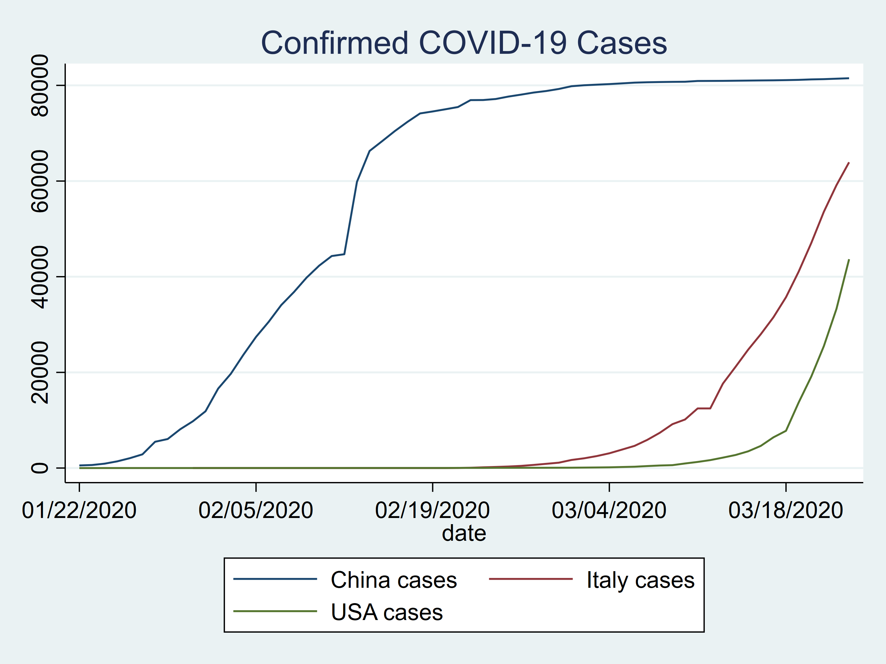
We could plot our data to compare the number of confirmed cases for China, Italy, and the US.
twoway (line china_c date)     ///

       (line italy_c date)     ///

       (line usa_c   date)      ///

       , title(Confirmed COVID-19 Cases)
Figure 2: Confirmed COVID-19 cases in China, Italy, and the US
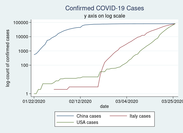
Many people prefer to plot their data on a log scale. This is easy to do using the yscale(log) option in our twoway command.
twoway (line china_c date)                                       ///

       (line italy_c date)                                               ///

       (line usa_c   date)                                               ///

       , title(Confirmed COVID-19 Cases)                     ///

       subtitle(y axis on log scale)                            ///

       ytitle(log-count of confirmed cases)                ///

       yscale(log)                                                              ///

       ylabel(0 100 1000 10000 100000, angle(horizontal))
Figure 3: Confirmed COVID-19 cases in China, Italy, and the United States plotted on a log scale
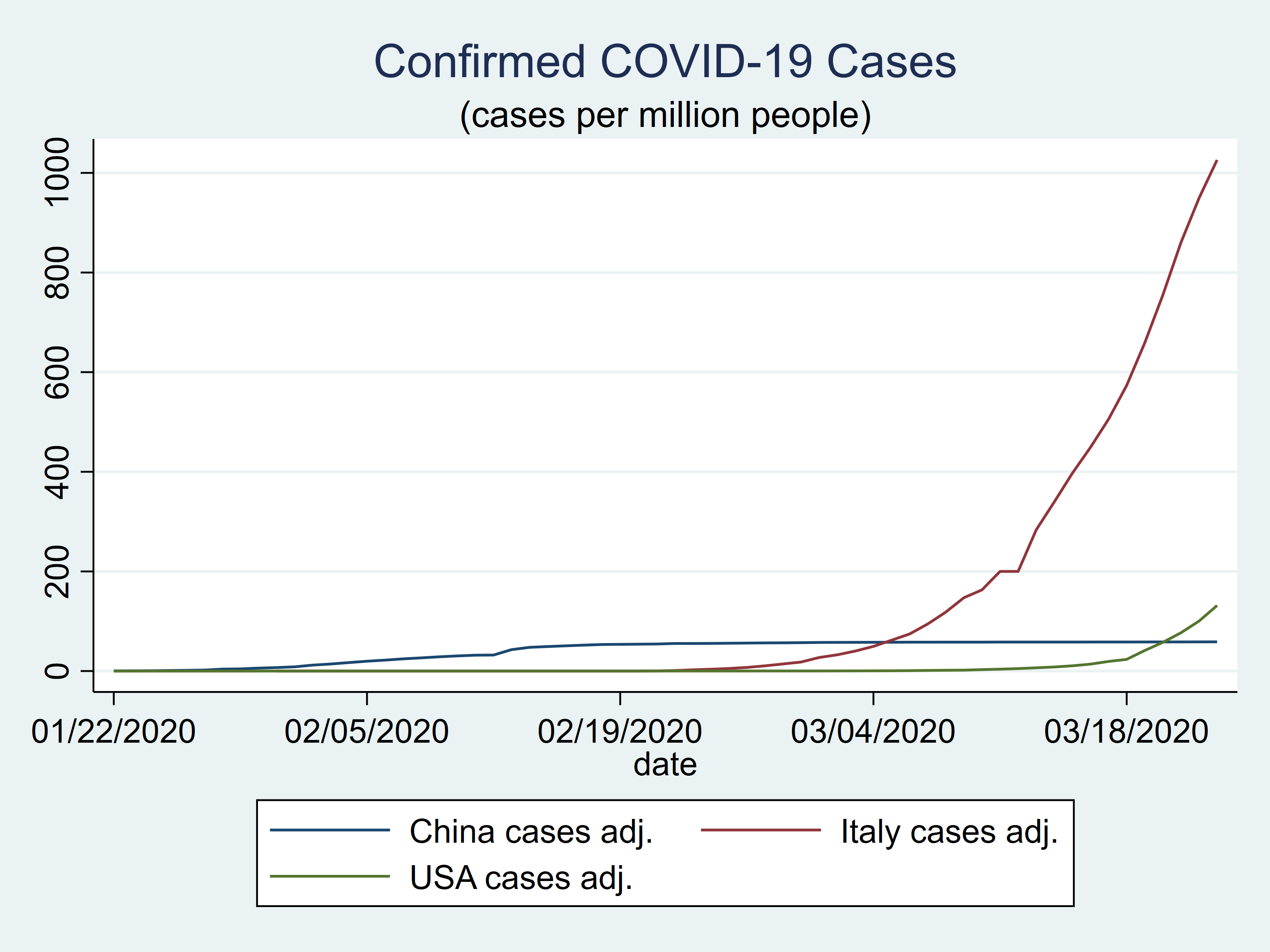
Using raw counts can be misleading because the populations of China, Italy, and the United States are quite different. Let’s create new variables that contain the number of confirmed cases per million population. The population data come from the United States Census Burea Population Clock.
generate china_ca = china_c / 1389.6

generate italy_ca = italy_c / 62.3

generate usa_ca   = usa_c / 331.8

label var china_ca "China cases adj."

label var italy_ca "Italy cases adj."

label var usa_ca "USA cases adj."

format %9.0f china_ca italy_ca usa_ca
The plot of the population-adjusted data looks quite different from the plot of the unadjusted data.
twoway (tsline china_ca)                       ///

       (tsline italy_ca)                       ///

       (tsline usa_ca)                         ///

       , title(Confirmed COVID-19 Cases)       ///

       subtitle("(cases per million people)")
Figure 4: Confirmed COVID-19 cases in China, Italy, and the United States adjusted for population size
We can add notes to our dataset to document the calculations for the population-adjusted data and the source of the population data.
notes china_ca: china_ca = china_c / 1389.6

notes china_ca: Population data source: https://www.census.gov/popclock/

notes italy_ca: italy_ca = italy_c / 62.3

notes italy_ca: Population data source: https://www.census.gov/popclock/

notes usa_ca:   usa_ca = usa_c / 331.8

notes usa_ca:   Population data source: https://www.census.gov/popclock/
We can view the notes by typing notes.
. notes

china_ca:
  1.  china_ca = china_c / 1389.6
  2.  Population data source: https://www.census.gov/popclock/

italy_ca:
  1.  italy_ca = italy_c / 62.3
  2.  Population data source: https://www.census.gov/popclock/

usa_ca:
  1.  usa_ca = usa_c / 331.8
  2.  Population data source: https://www.census.gov/popclock/
We can also label our dataset and add notes for the entire dataset.
label data "COVID-19 Data assembled for the Stata Blog"

notes _dta: Raw data course: https://github.com/CSSEGISandData/COVID-19/tree/master/csse_covid_19_data/csse_covid_19_daily_reports

notes _dta: These data are for instructional purposes only
Last, we can tsset and save our dataset.
. tsset date, daily
        time variable:  date, 01/22/2020 to 03/23/2020
                delta:  1 day

. save covid19_wide, replace
file covid19_wide.dta saved
Conclusion and combined commands
We did it! We successfully downloaded the raw data files, merged them, formatted them, and created two datasets that we can use to make tables and graphs. It would have been easier if the data were formatted consistently over time, but that is the nature of real data. Fortunately, we have the tools and skills we need to handle these kinds of tasks. I’ve collected the Stata commands below so you can run them all at once if you like. The raw data may change again in the future, and you may need to modify the code below to handle those changes.
I would again like to strongly emphasize that we have not checked and cleaned these data. The code and the resulting data should be used for instructional purposes only.
Stata code to download COVID-19 data from Johns Hopkins University as of March 23, 2020
local URL = "https://raw.githubusercontent.com/CSSEGISandData/COVID-19/master/csse_covid_19_data/csse_covid_19_daily_reports/"

forvalues month = 1/12 {

   forvalues day = 1/31 {

      local month = string(`month', "%02.0f")

      local day = string(`day', "%02.0f")

      local year = "2020"

      local today = "`month'-`day'-`year'"

      local FileName = "`URL'`today'.csv"

      clear

      capture import delimited "`FileName'"

capture confirm variable ïprovincestate

      if _rc == 0 {

         rename ïprovincestate provincestate

         label variable provincestate "Province/State"

      }

      capture rename province_state provincestate

      capture rename country_region countryregion

      capture rename last_update lastupdate

      capture rename lat latitude

      capture rename long longitude

      generate tempdate = "`today'"

      capture save "`today'", replace

   }

}

clear

forvalues month = 1/12 {

   forvalues day = 1/31 {

      local month = string(`month', "%02.0f")

      local day = string(`day', "%02.0f")

      local year = "2020"

      local today = "`month'-`day'-`year'"

      capture append using "`today'"

   }

}

generate date = date(tempdate, "MDY")

format date %tdNN/DD/CCYY
replace countryregion = "China" if countryregion=="Mainland China"

keep if inlist(countryregion, "China", "US", "Italy")

collapse (sum) confirmed deaths recovered, by(date countryregion)

encode countryregion, gen(country)

tsset country date, daily

save covid19_long, replace
keep date country confirmed deaths recovered

reshape wide confirmed deaths recovered, i(date) j(country)

rename confirmed1 china_c

rename deaths1    china_d

rename recovered1 china_r

label var china_c "China cases"

label var china_d "China deaths"

label var china_r "China recovered"

rename confirmed2 italy_c

rename deaths2    italy_d

rename recovered2 italy_r

label var italy_c "Italy cases"

label var italy_d "Italy deaths"

label var italy_r "Italy recovered"

rename confirmed3 usa_c

rename deaths3    usa_d

rename recovered3 usa_r

label var usa_c "USA cases"

label var usa_d "USA deaths"

label var usa_r "USA recovered"

generate china_ca = china_c / 1389.6

generate italy_ca = italy_c / 62.3

generate usa_ca   = usa_c / 331.8

label var china_ca "China cases adj."

label var italy_ca "Italy cases adj."

label var usa_ca "USA cases adj."

format %9.0f china_ca italy_ca usa_ca

notes china_ca: china_ca = china_c / 1389.6

notes china_ca: Population data source: https://www.census.gov/popclock/

notes italy_ca: italy_ca = italy_c / 62.3

notes italy_ca: Population data source: https://www.census.gov/popclock/

notes usa_ca:   usa_ca = usa_c / 331.8

notes usa_ca:   Population data source: https://www.census.gov/popclock/

label data "COVID-19 Data assembled for the Stata Blog"

notes _dta: Raw data course: https://github.com/CSSEGISandData/COVID-19/tree/master/csse_covid_19_data/csse_covid_19_daily_reports

notes _dta: These data are for instructional purposes only

tsset date, daily

save covid19_wide, replace