How to create choropleth maps using the COVID-19 data from Johns Hopkins University
In my last post, we learned how to import the raw COVID-19 data from the Johns Hopkins GitHub repository and convert the raw data to time-series data. This post will demonstrate how to download raw data and create choropleth maps like figure 1.
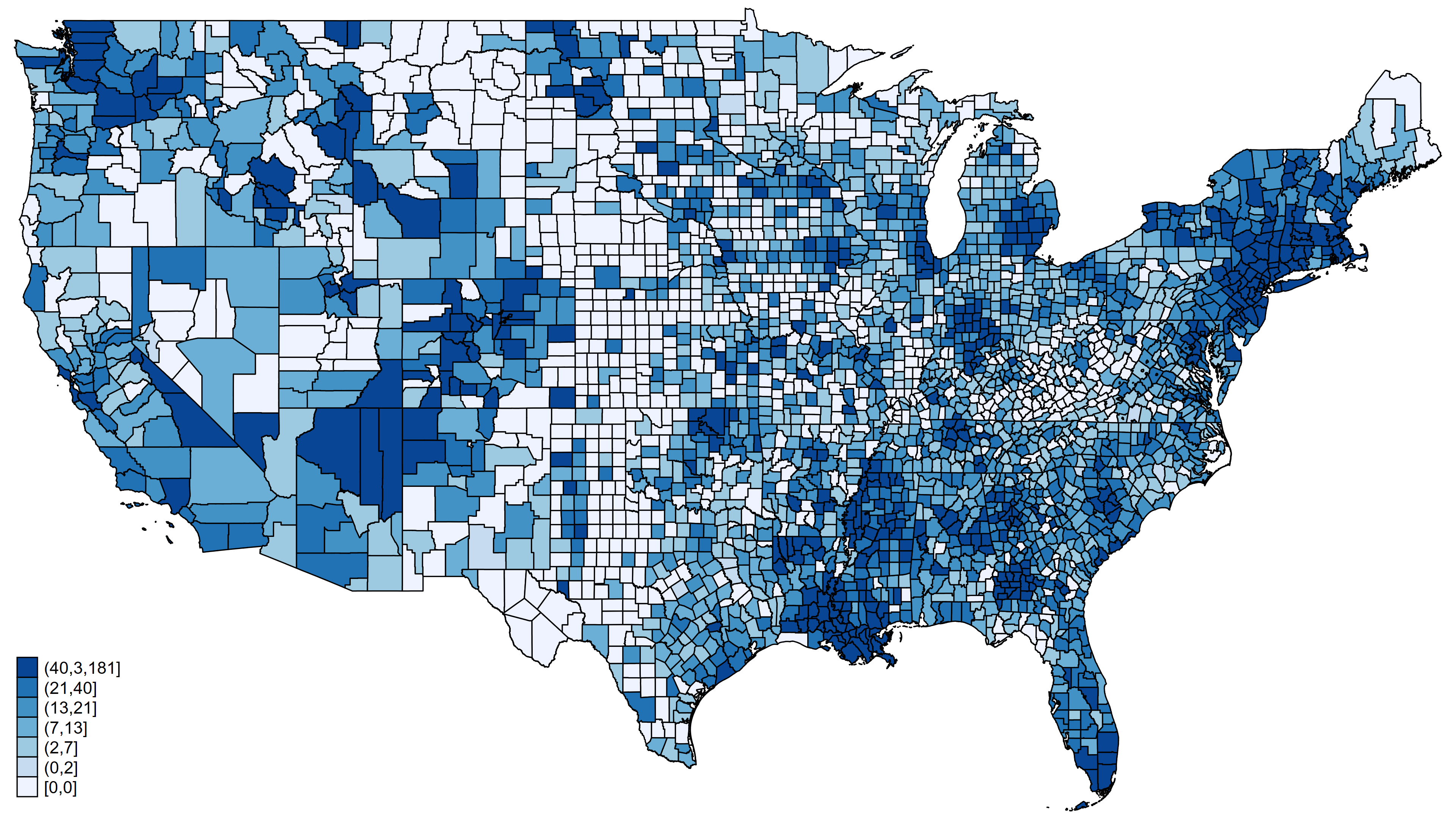
Figure 1: Confirmed COVID-19 cases in United States adjusted for population size
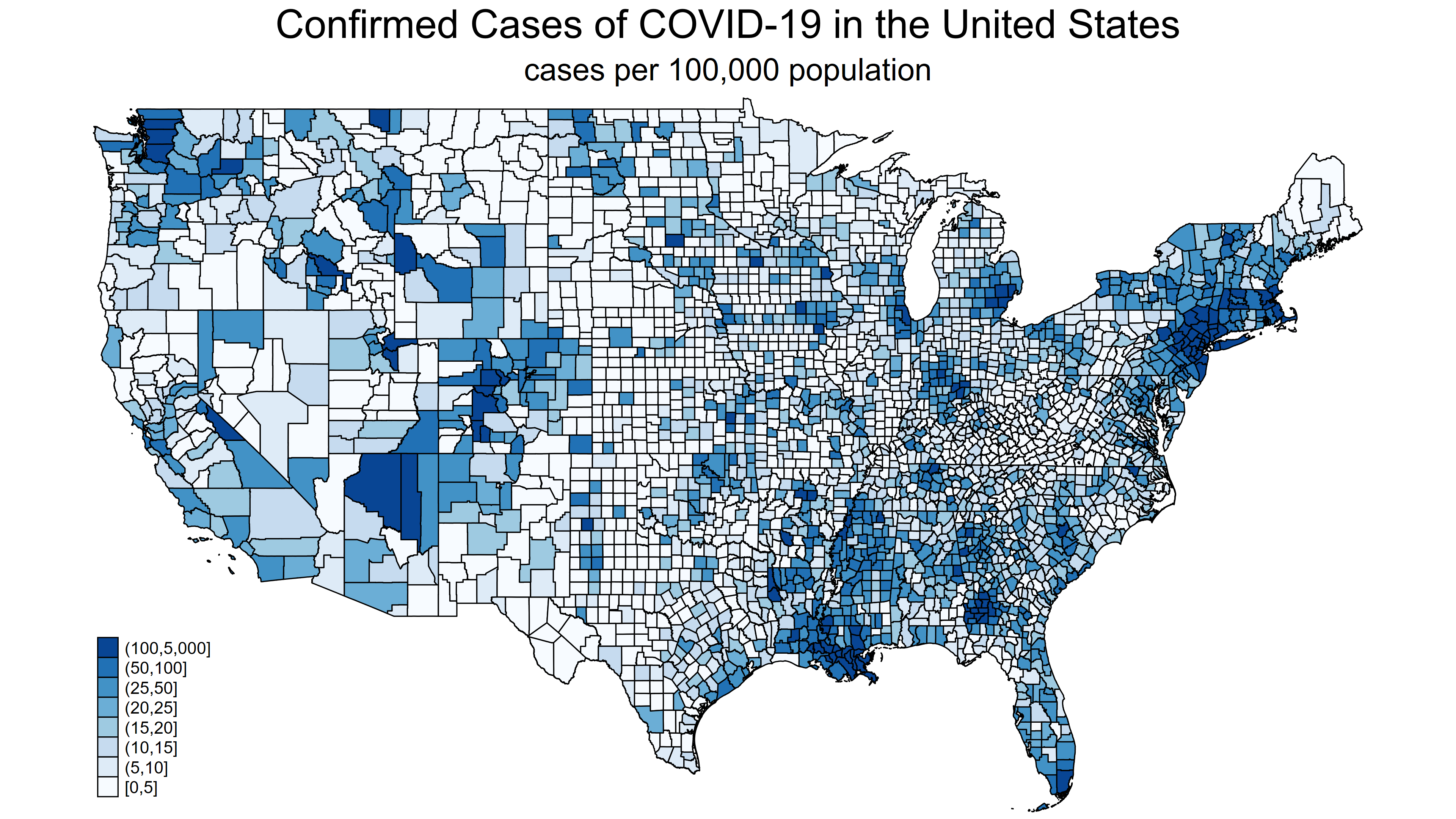
A choropleth map displays statistical information about geographical areas using different colors or shading intensity. Figure 1 displays the population-adjusted number of confirmed cases of COVID-19 for each county in the United States as of April 2, 2020. Each shade of blue on the map represents the range of the number of cases shown in the legend at the bottom left of the map. I used the community-contributed command grmap to create figure 1, and we need three pieces of information about each county to create this map. We need the geographic information for each county, the number of confirmed cases in each county, and the population of each county.
Let begin at the end and work our way backward to learn how to construct a dataset that contains this information. The data listed below were used to create the map in figure 1. Each observation contains information about an individual county in the United States.
. list _ID GEOID _CX _CY confirmed popestimate2019 confirmed_adj ///
      in 1/5, abbrev(12)

     +------------------------------------------------------------------------+
     | _ID   GEOID      _CX     _CY   confirmed   popesti~2019   confirmed_~j |
     |------------------------------------------------------------------------|
  1. |   1   21007   -89.00   37.06           0           7888              0 |
  2. |   2   21017   -84.22   38.21           2          19788             10 |
  3. |   3   21031   -86.68   37.21           1          12879              8 |
  4. |   4   21065   -83.96   37.69           0          14106              0 |
  5. |   5   21069   -83.70   38.37           0          14581              0 |
     +------------------------------------------------------------------------+
The first four variables contain geographic information about each county. The variable _ID contains a unique identification number for each county that is used to link with a special file called a “shapefile”. Shapefiles contain the information that is used to render the map and will be explained below. The variable GEOID is a Federal Information Processing Standard (FIPS) county code. We can use the FIPS code as a key variable to merge data from other files. The variables _CX and _CY contain geographic coordinates. We can download these data from the United States Census Bureau.
The variable confirmed contains the number of confirmed cases of COVID-19 in each county. These data were downloaded from the Johns Hopkins GitHub repository. This is not the same file that we used in my previous posts.
The variable popestimate2019 contains the population of each county. These data were downloaded from the United States Census Bureau.
The variable confirmed_adj contains the number of confirmed cases per 100,000 population. This variable is calculated by dividing the number of cases for each county in confirmed by the total population for each county in popestimate2019. The result is multiplied by 100,000 to convert to “cases per 100,000 population”.
We will need to download data from three different sources and merge these files into a single dataset to construct the dataset for our map. Let’s begin by downloading and processing each of these datasets.
List of topics
Download and prepare the geographic data
Download and prepare the case data
Download and prepare the population data
How to merge the files and calculate adjusted counts
How to create the choropleth map with grmap
Download and prepare the geographic data
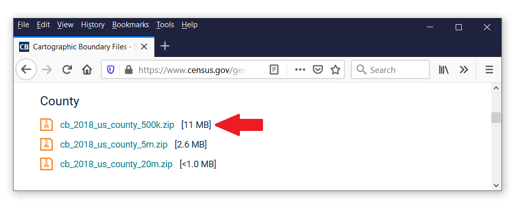
Let’s begin with the geographic data. Shapefiles contain the geographic information that grmap uses to create maps. Many shapefiles are available freely on the Internet, and you can locate them using a search engine. For example, I searched for the terms “united states shapefile”, and the first result took me to the United States Census Bureau. This website contains shapefiles for the United States that show boundaries for states, congressional districts, metropolitan, micropolitan statistical areas, and many others. I would like to subdivide my map of the United States by county, so I scrolled down until I found the heading “County”. I would like to use the file cb_2018_us_county_500k.zip.
We can copy the file from the website to our local drive and use unzipfile to extract the contents of the file. You can right-click on the file on the webpage, select “Copy Link Location”, and paste the path and filename to your copy command.
. copy https://www2.census.gov/geo/tiger/GENZ2018/shp/cb_2018_us_county_500k.zip ///
>      cb_2018_us_county_500k.zip

. unzipfile cb_2018_us_county_500k.zip
    inflating: cb_2018_us_county_500k.shp.ea.iso.xml
    inflating: cb_2018_us_county_500k.shp.iso.xml
    inflating: cb_2018_us_county_500k.shp
    inflating: cb_2018_us_county_500k.shx
    inflating: cb_2018_us_county_500k.dbf
    inflating: cb_2018_us_county_500k.prj
    inflating: cb_2018_us_county_500k.cpg

successfully unzipped cb_2018_us_county_500k.zip to current directory
total processed:  7
        skipped:  0
      extracted:  7
The files cb_2018_us_county_500k.shp and cb_2018_us_county_500k.dbf contain the geographic information we need. We can use spshape2dta to process the information in these files and create two Stata datasets named usacounties_shp.dta and usacounties.dta.
. spshape2dta cb_2018_us_county_500k.shp, saving(usacounties) replace
  (importing .shp file)
  (importing .dbf file)
  (creating _ID spatial-unit id)
  (creating _CX coordinate)
  (creating _CY coordinate)

  file usacounties_shp.dta created
  file usacounties.dta     created
The file usacounties_shp.dta is the shapefile that contains the information that grmap will use to render the map. We don’t need to do anything to this file, but let’s describe and list its contents to see what it contains.
. use usacounties_shp.dta, clear

. describe

Contains data from usacounties_shp.dta
  obs:     1,047,409
 vars:             5                          3 Apr 2020 10:36
----------------------------------------------------------------------
              storage   display    value
variable name   type    format     label      variable label
----------------------------------------------------------------------
_ID             int     %12.0g
_X              double  %10.0g
_Y              double  %10.0g
rec_header      strL    %9s
shape_order     int     %12.0g
----------------------------------------------------------------------
Sorted by: _ID

. list _ID _X _Y shape_order in 1/10, abbreviate(11)

     +--------------------------------------------+
     | _ID           _X          _Y   shape_order |
     |--------------------------------------------|
  1. |   1            .           .             1 |
  2. |   1   -89.181369   37.046305             2 |
  3. |   1   -89.179384   37.053012             3 |
  4. |   1   -89.175725   37.062069             4 |
  5. |   1   -89.171881   37.068184             5 |
     |--------------------------------------------|
  6. |   1   -89.168087   37.074218             6 |
  7. |   1   -89.167029   37.075362             7 |
  8. |   1   -89.154504   37.088907             8 |
  9. |   1   -89.154311   37.089002             9 |
 10. |   1   -89.151294   37.090487            10 |
     +--------------------------------------------+
The shapefile, usacounties_shp.dta, contains 1,047,409 coordinates that define the boundaries of each county on our map. This file also includes the variable _ID, which is used to link these data with the data in usacounties.dta. We will need this file later.
Next, let’s use and describe the contents of usacounties.dta.
. use usacounties.dta, clear

. describe

Contains data from usacounties.dta
  obs:         3,233
 vars:            12                          3 Apr 2020 10:36
---------------------------------------------------------------------------
              storage   display    value
variable name   type    format     label      variable label
---------------------------------------------------------------------------
_ID             int     %12.0g                Spatial-unit ID
_CX             double  %10.0g                x-coordinate of area centroid
_CY             double  %10.0g                y-coordinate of area centroid
STATEFP         str2    %9s                   STATEFP
COUNTYFP        str3    %9s                   COUNTYFP
COUNTYNS        str8    %9s                   COUNTYNS
AFFGEOID        str14   %14s                  AFFGEOID
GEOID           str5    %9s                   GEOID
NAME            str21   %21s                  NAME
LSAD            str2    %9s                   LSAD
ALAND           double  %14.0f                ALAND
AWATER          double  %14.0f                AWATER
---------------------------------------------------------------------------
Sorted by: _ID
The first three variables contain geographic information about each state. The variable _ID is the spatial-unit identifier for each county that is used to link this file with the shapefile, usacounties_shp.dta. The variables _CX and _CY are the x and y coordinates of the area centroid for each county. The variable NAME contains the name of the county for each observation. The variable GEOID is the FIPS code stored as a string. We will need a numeric FIPS code to merge this dataset with other county-level datasets. So let’s generate a variable named fips that equals the numeric value of GEOID.
. generate fips = real(GEOID)

. list _ID GEOID fips NAME in 1/10, separator(0)

     +-------------------------------+
     | _ID   GEOID    fips      NAME |
     |-------------------------------|
  1. |   1   21007   21007   Ballard |
  2. |   2   21017   21017   Bourbon |
  3. |   3   21031   21031    Butler |
  4. |   4   21065   21065    Estill |
  5. |   5   21069   21069   Fleming |
  6. |   6   21093   21093    Hardin |
  7. |   7   21099   21099      Hart |
  8. |   8   21131   21131    Leslie |
  9. |   9   21151   21151   Madison |
 10. |  10   21155   21155    Marion |
     +-------------------------------+
Let’s save our geographic data and move on to the COVID-19 data.
. save usacounties.dta
file usacounties.dta saved
Download and prepare the case data
In my previous posts, we learned how to download the raw COVID-19 data from the Johns Hopkins GitHub repository. We will use a different dataset from another branch of the GitHub repository located here.
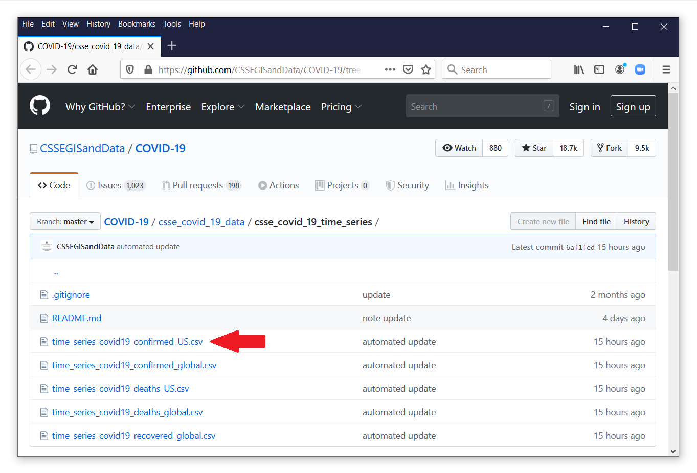
The file time_series_covid19_confirmed_US.csv contains time-series data for the number of confirmed cases of COVID-19 for each county in the United States. Let’s click on the filename to view its contents.
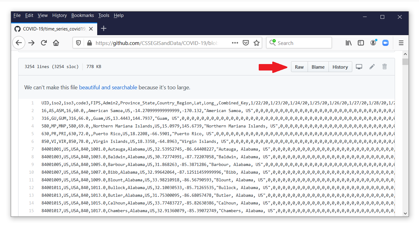
Each observation in this file contains the data for a county or territory in the United States. The confirmed counts for each date are stored in separate variables. Let’s view the comma-delimited data by clicking on the button labeled “Raw” next to the red arrow.
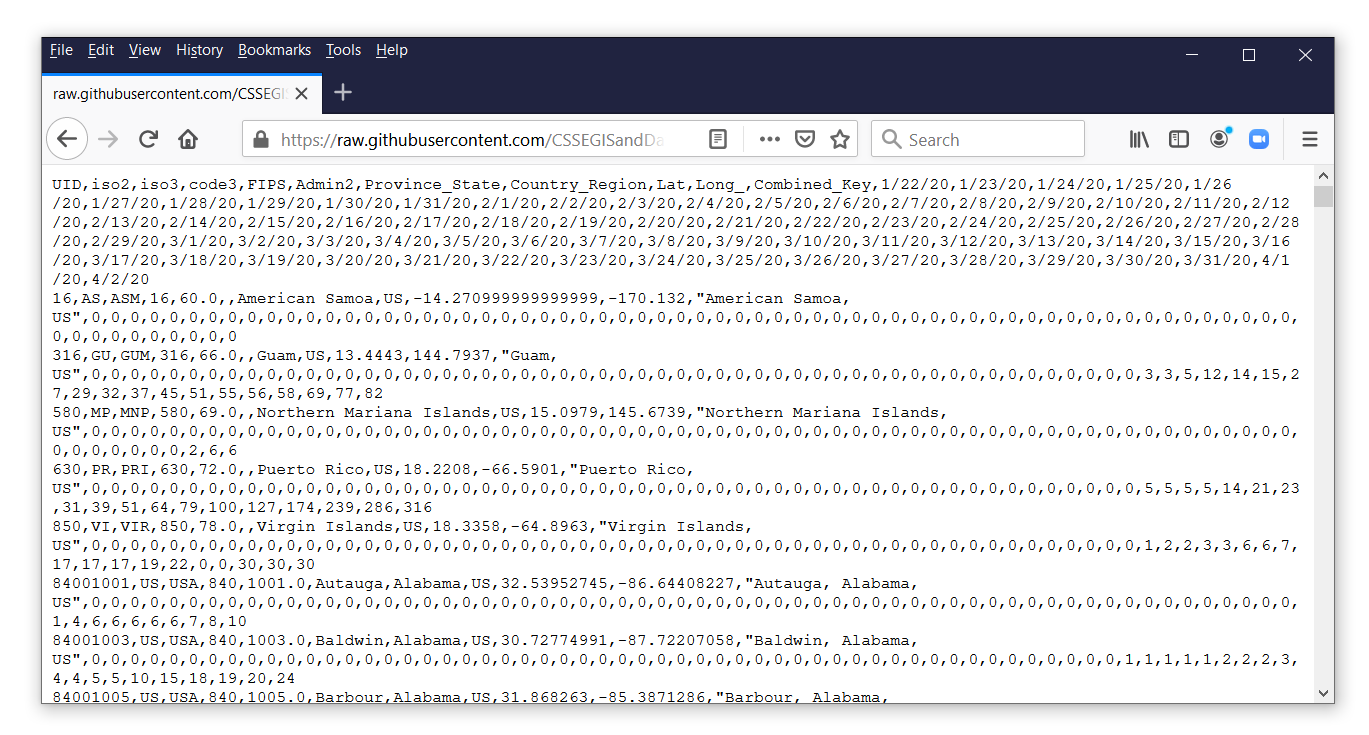
To import the raw case data, copy the URL and the filename from the address bar in your web browser, and paste the web address into import delimited.
. import delimited
> https://raw.githubusercontent.com/CSSEGISandData/COVID-19/
> master/csse_covid_19_data/csse_covid_19_time_series/
> time_series_covid19_confirmed_US.csv
(83 vars, 3,253 obs)
Note that the URL for the data file is long and wraps to a second and third line in our import delimited command. This URL must be one line in your import delimited command. Let’s describe this dataset.
. describe

Contains data
  obs:         3,253
 vars:            83
----------------------------------------------------------------------
              storage   display    value
variable name   type    format     label      variable label
----------------------------------------------------------------------
uid             long    %12.0g                UID
iso2            str2    %9s
iso3            str3    %9s
code3           int     %8.0g
fips            long    %12.0g                FIPS
admin2          str21   %21s                  Admin2
province_state  str24   %24s                  Province_State
country_region  str2    %9s                   Country_Region
lat             float   %9.0g                 Lat
long_           float   %9.0g                 Long_
combined_key    str44   %44s                  Combined_Key
v12             byte    %8.0g                 1/22/20
v13             byte    %8.0g                 1/23/20
v14             byte    %8.0g                 1/24/20
v15             byte    %8.0g                 1/25/20

               (Output omitted)

v80             long    %12.0g                3/30/20
v81             long    %12.0g                3/31/20
v82             long    %12.0g                4/1/20
v83             long    %12.0g                4/2/20
----------------------------------------------------------------------
Sorted by:
This dataset contains 3,253 observations that contain information about counties in the United States. Let’s list the first 10 observations for fips, combined_key, v80, v81, v82, and v83.
. list fips combined_key v80 v81 v82 v83 in 1/10

     +-------------------------------------------------------------+
     | fips                   combined_key   v80   v81   v82   v83 |
     |-------------------------------------------------------------|
  1. |   60             American Samoa, US     0     0     0     0 |
  2. |   66                       Guam, US    58    69    77    82 |
  3. |   69   Northern Mariana Islands, US     0     2     6     6 |
  4. |   72                Puerto Rico, US   174   239   286   316 |
  5. |   78             Virgin Islands, US     0    30    30    30 |
     |-------------------------------------------------------------|
  6. | 1001           Autauga, Alabama, US     6     7     8    10 |
  7. | 1003           Baldwin, Alabama, US    18    19    20    24 |
  8. | 1005           Barbour, Alabama, US     0     0     0     0 |
  9. | 1007              Bibb, Alabama, US     2     3     3     4 |
 10. | 1009            Blount, Alabama, US     5     5     5     6 |
     +-------------------------------------------------------------+
The variable fips contains the FIPS county code that we will use to merge this dataset with the geographic information in usacounties_shp.dta. The variable combined_key contains the name of each county and state in the United States. And the variables v80, v81, v82, and v83 contain the number of confirmed cases of COVID-19 from March 30, 2020, through April 2, 2020. The most recent case data are stored in v83, so let’s change its name to confirmed.
. rename v83 confirmed
We will encounter problems later when we merge datasets if fips contains missing values. So let’s drop any observations that are missing data for fips.
. drop if missing(fips)
(2 observations deleted)
Our COVID-19 dataset is complete. Let’s save the data and move on to the population data.
. save covid19_adj, replace
file covid19_adj.dta saved
Download and prepare the population data
We could stop here, merge the geographic data with the number of confirmed cases, and create a choropleth map of the number of cases for each county. But this would be misleading because the populations of the counties are different. We might prefer to report the number of cases per 100,000 people, and that would require knowing the number of people in each county. Fortunately, those data are available on the United States Census Bureau website.
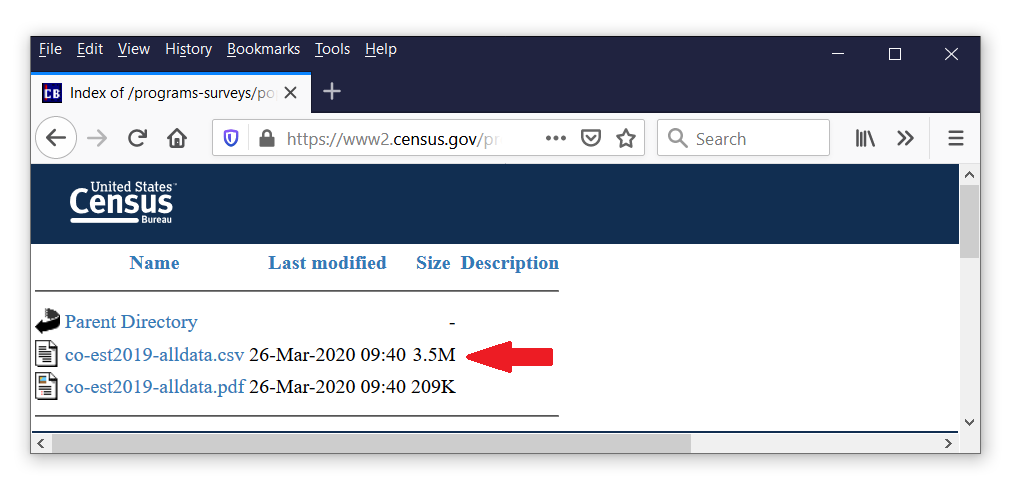
We can follow the same steps we used to download and import the case data. First, right-click on the filename on the website, then select “Copy Link Location”, and use import delimited to import the data.
. import delimited https://www2.census.gov/programs-surveys/popest/datasets/
> 2010-2019/counties/totals/co-est2019-alldata.csv
(164 vars, 3,193 obs)
I would typically describe the dataset at this point, but there are 164 variables in this dataset. So I will describe only the relevant variables below.
. describe state county stname ctyname census2010pop popestimate2019

              storage   display    value
variable name   type    format     label      variable label
----------------------------------------------------------------------
state           byte    %8.0g                 STATE
county          int     %8.0g                 COUNTY
stname          str20   %20s                  STNAME
ctyname         str33   %33s                  CTYNAME
census2010pop   long    %12.0g                CENSUS2010POP
popestimate2019 long    %12.0g                POPESTIMATE2019
The variable census2010pop contains the population of each county based on the 2010 census. But that information is 10 years old. The variable popestimate2019 is an estimate of the population of each county in 2019. Let’s use those data because they are more recent.
Next, let’s list the data.
. list state county stname ctyname census2010pop popestimate2019 ///
      in 1/5, abbreviate(14) noobs

  +----------------------------------------------------------------------------+
  | state   county    stname          ctyname   census2010pop   popestima~2019 |
  |----------------------------------------------------------------------------|
  |     1        0   Alabama          Alabama         4779736          4903185 |
  |     1        1   Alabama   Autauga County           54571            55869 |
  |     1        3   Alabama   Baldwin County          182265           223234 |
  |     1        5   Alabama   Barbour County           27457            24686 |
  |     1        7   Alabama      Bibb County           22915            22394 |
  +----------------------------------------------------------------------------+
This dataset does not include a variable with a FIPS county code. But we can create a variable that contains the FIPS code using the variables state and county. Visual inspection of the geographic data in usacounties.dta indicates that the FIPS county code is the state code followed by the three-digit state code. So let’s create our fips code variable by multiplying the state code by 1000 and then adding the county code.
. generate fips = state*1000 + county
Let’s list the county data to check our work.
. list state county fips stname ctyname ///
      in 1/5, abbreviate(14) noobs

  +--------------------------------------------------+
  | state   county   fips    stname          ctyname |
  |--------------------------------------------------|
  |     1        0   1000   Alabama          Alabama |
  |     1        1   1001   Alabama   Autauga County |
  |     1        3   1003   Alabama   Baldwin County |
  |     1        5   1005   Alabama   Barbour County |
  |     1        7   1007   Alabama      Bibb County |
  +--------------------------------------------------+
This dataset contains the estimated population of each state along with the variable fips that we will use as a key variable to merge this data file with the other data files. Let’s save our data.
. save census_popn, replace
file census_popn.dta saved
How to merge the files and calculate adjusted counts
We have created three data files that contain the information we need to create our choropleth map. The data file usacounties.dta contains the geographic information we need in the variables _ID, _CX, and _CY. Recall that these data are linked to the shapefile, usacounties_shp.dta, using the variable _ID. The data file covid19_county.dta contains the information about the number of confirmed cases of COVID-19 in the variable confirmed. And the data file census_popn.dta contains the information about the population for each county in the variable popestimate2019.
We need all of these variables in the same dataset to create our map. We can merge these files using the key variable fips.
Let’s begin by using only the variables we need from usacounties.dta.
. use _ID _CX _CY GEOID fips using usacounties.dta
Next, let’s merge the number of confirmed cases from covid19_county.dta. The option keepusing(province_state combined_key confirmed) specifies that we will merge only the variables province_state, combined_key, and confirmed from the data file covid19_state.dta.
. merge 1:1 fips using covid19_county  ///
       , keepusing(province_state combined_key confirmed)
(note: variable fips was float, now double to accommodate using data's values)

    Result                           # of obs.
    -----------------------------------------
    not matched                           200
        from master                        91  (_merge==1)
        from using                        109  (_merge==2)

    matched                             3,142  (_merge==3)
    -----------------------------------------
The output tells us that 3,142 observations had matching values of fips in the two datasets. merge also created a new variable in our dataset named _merge, which equals 3 for observations with matching values of fips.
The output also tells us that 91 observations had a fips code in the geographic data but not in the case data. _merge equals 1 for these observations. Let’s list some of these observations.
. list _ID GEOID fips combined_key confirmed ///
      if _merge==1, abbreviate(15)

      +-------------------------------------------------+
      |  _ID   GEOID    fips   combined_key   confirmed |
      |-------------------------------------------------|
3143. |  502   60010   60010                          . |
3144. |  503   60020   60020                          . |
3145. | 1475   60030   60030                          . |
3146. | 1476   60040   60040                          . |
3147. | 1068   60050   60050                          . |
      |-------------------------------------------------|
3148. | 1210   66010   66010                          . |
3149. |  504   69085   69085                          . |
        (Output omitted)
The first seven observations have geographic information but no data for confirmed. Let’s
count the number of observations where _merge equals 1 and the data are missing for confirmed.
. count if _merge==1 & missing(confirmed)
  91
Let’s drop these observations from our dataset because they contain no data for confirmed.
. drop if _merge==1
(91 observations deleted)
The merge output also tells us that 109 observations had a fips code in the case data but not in the geographic data. _merge equals 2 for these observations. Let’s list some of these observations.
. list _ID GEOID fips combined_key confirmed ///
      if _merge==2, abbreviate(15)

      +------------------------------------------------------------------------+
      | _ID   GEOID    fips                           combined_key   confirmed |
      |------------------------------------------------------------------------|
3143. |   .              60                     American Samoa, US           0 |
3144. |   .              66                               Guam, US          82 |
3145. |   .              69           Northern Mariana Islands, US           6 |
3146. |   .              72                        Puerto Rico, US         316 |
3147. |   .              78                     Virgin Islands, US          30 |
      |------------------------------------------------------------------------|
3148. |   .           80001                 Out of AL, Alabama, US           0 |
3149. |   .           80002                  Out of AK, Alaska, US           0 |
The first seven observations have case information but no data for _ID or GEOID.
Some of the observations are from American territories that are not states. Other observations have a value of combined_key that suggests that the county information is not clear. Visual inspection of these observations suggests that most of the confirmed cases for these observations are zero. We can verify this by counting the number of observations where _merge equals 2 and confirmed equals zero.
. count if _merge==2 & confirmed==0
  78
The output indicates that 78 of the 109 observations contain no confirmed cases. We could investigate these observations further if we were using our results to make policy decisions. But these observations are a small proportion of our dataset, and our present goal is only to learn how to make choropleth maps. So let’s delete these observations and the variable _merge and move on.
. drop if _merge==2
(109 observations deleted)

. drop _merge
Let’s describe the dataset to verify that merge was successful.
. describe

Contains data from usacounties.dta
  obs:         3,142
 vars:             8                          3 Apr 2020 15:55
---------------------------------------------------------------------------
              storage   display    value
variable name   type    format     label      variable label
---------------------------------------------------------------------------
_ID             int     %12.0g                Spatial-unit ID
_CX             double  %10.0g                x-coordinate of area centroid
_CY             double  %10.0g                y-coordinate of area centroid
GEOID           str5    %9s                   GEOID
fips            double  %9.0g
province_state  str24   %24s                  Province_State
combined_key    str44   %44s                  Combined_Key
confirmed       long    %12.0g                4/2/20
---------------------------------------------------------------------------
Sorted by:
Next, let’s merge the variable popestimate2019 from the data file census_popn.dta.
. merge 1:1 fips using census_popn

    Result                           # of obs.
    -----------------------------------------
    not matched                            51
        from master                         0  (_merge==1)
        from using                         51  (_merge==2)

    matched                             3,142  (_merge==3)
    -----------------------------------------
The output tells us that 3,142 observations had matching values of fips in the two datasets. merge again created a new variable in our dataset named _merge, which equals 3 for observations with a matching value of fips.
The output also tells us that 51 observations had a fips code in the geographic data but not in the population data. _merge equals 2 for these observations. Let’s list some of these observations.
. list _ID GEOID fips combined_key confirmed popestimate2019 ///
      if _merge==2, abbreviate(15)

      +------------------------------------------------------------------+
      | _ID   GEOID    fips   combined_key   confirmed   popestimate2019 |
      |------------------------------------------------------------------|
3143. |   .            1000                          .           4903185 |
3144. |   .            2000                          .            731545 |
3145. |   .            4000                          .           7278717 |
3146. |   .            5000                          .           3017804 |
3147. |   .            6000                          .          39512223 |
      |------------------------------------------------------------------|
3148. |   .            8000                          .           5758736 |
3149. |   .            9000                          .           3565287 |
We have no geographic or case information for these observations, so let’s drop them from our dataset as well as drop the variable _merge.
. keep if _merge==3
(51 observations deleted)

. drop _merge
Now, let’s generate, label, and format a new variable named confirmed_adj that contains the population-adjusted number of confirmed COVID-19 cases.
. generate confirmed_adj = 100000*(confirmed/popestimate2019)

. label var confirmed_adj "Cases per 100,000"

. format %16.0fc confirmed_adj
Let’s describe our dataset to verify that it contains all the variables we will need to create our map.
. describe

Contains data from usacounties.dta
  obs:         3,142
 vars:            10                          3 Apr 2020 14:15
---------------------------------------------------------------------------
              storage   display    value
variable name   type    format     label      variable label
---------------------------------------------------------------------------
_ID             int     %12.0g                Spatial-unit ID
_CX             double  %10.0g                x-coordinate of area centroid
_CY             double  %10.0g                y-coordinate of area centroid
GEOID           str5    %9s                   GEOID
fips            double  %9.0g
combined_key    str44   %44s                  Combined_Key
confirmed       long    %12.0g                4/2/20
census2010pop   long    %12.0g                CENSUS2010POP
popestimate2019 long    %12.0g                POPESTIMATE2019
confirmed_adj   float   %16.0fc               Cases per 100,000
---------------------------------------------------------------------------
Sorted by:
Our dataset is complete! Let’s save the dataset and learn how to create a choropleth map.
. save covid19_adj
file covid19_adj.dta saved
How to create the choropleth map with grmap
We will use the community-contributed command grmap to create our choropleth map. You must activate grmap before you use it for the first time.
. grmap, activate
Creating a map that includes Alaska and Hawaii will require the use of options that adjust for their large difference in size and for their not being physically adjacent to the other 48 states. I would like to keep our map as simple as possible for now, so I am going to drop the observations for Alaska and Hawaii.
. drop if inlist(NAME, "Alaska", "Hawaii")
(2 observations deleted)
Next, we must tell Stata that these are spatial data by using spset. The option modify shpfile(usastates_shp) will link our data with the shapefile, usastates_shp.dta. Recall that the shapefile contains the information that grmap will use to render the map.
. spset, modify shpfile(usacounties_shp)
  (creating _ID spatial-unit id)
  (creating _CX coordinate)
  (creating _CY coordinate)
  Sp dataset covid19_adj.dta
                data:  cross sectional
     spatial-unit id:  _ID
         coordinates:  _CX, _CY (planar)
    linked shapefile:  usacounties_shp.dta
Now, we can use grmap to create a choropleth map for the population-adjusted number of confirmed cases of COVID-19.
. grmap confirmed_adj, clnumber(7)
Figure 2: Choropleth map using sectiles
By default, grmap divides the data into four groups based on quartiles of confirmed_adj. I have used the option clnumber(7) to divide the data into 7 groups or sectiles. You can change the number of groups using the clnumber(#) option, where # is the number of color categories.
You can also specify custom cutpoints using the options clmethod(custom) and clbreaks(numlist). The map below uses custom cutpoints at 0, 5, 10, 15, 20, 25, 50, 100, and 5000. I have also added a title and a subtitle.
. grmap confirmed_adj,                                            ///
       clnumber(8)                                               ///
       clmethod(custom)                                          ///
       clbreaks(0 5 10 15 20 25 50 100 5000)                     ///
       title("Confirmed Cases of COVID-19 in the United States") ///
       subtitle("cases per 100,000 population")
Figure 3: Choropleth map using custom cutpoints
Conclusion and collected code
We did it! We created a choropleth map of the population-adjusted number of confirmed COVID-19 cases in each county of the United States! Let’s review the basic steps. First, we downloaded the geographic data from the United States Census Bureau and converted them to Stata data files using spshape2dta. Second, we downloaded, imported, and processed the COVID-19 data from the Johns Hopkins GitHub repository and saved the data to a Stata data file. Third, we downloaded, imported, and processed the population data for each county from the United States Census Bureau and saved the data to a Stata data file. Fourth, we merged the Stata data files and calculated the population-adjusted number of COVID-19 cases for each county. And fifth, we used spset to tell Stata that these are spatial data, and we used grmap to create our choropleth map. You could follow these steps to create a choropleth map for many kinds of data, for other subdivisions of the United States, or for other countries.
I have collected the code below that will reproduce figures 2 and 3.
// Create the geographic datasets

clear

copy https://www2.census.gov/geo/tiger/GENZ2018/shp/cb_2018_us_county_500k.zip ///

     cb_2018_us_county_500k.zip

unzipfile cb_2018_us_county_500k.zip

spshape2dta cb_2018_us_county_500k.shp, saving(usacounties) replace

use usacounties.dta, clear

generate fips = real(GEOID)

save usacounties.dta, replace
// Create the COVID-19 case dataset

clear

import delimited https://raw.githubusercontent.com/CSSEGISandData/COVID-19/master/csse_covid_19_data/csse_covid_19_time_series/time_series_covid19_confirmed_US.csv

rename v83 confirmed

drop if missing(fips)

save covid19_county, replace
// Create the population dataset

clear

import delimited https://www2.census.gov/programs-surveys/popest/datasets/2010-2019/counties/totals/co-est2019-alldata.csv

generate fips = state*1000 + county

save census_popn, replace
// Merge the datasets

clear

use _ID _CX _CY GEOID fips using usacounties.dta

merge 1:1 fips using covid19_county  ///

     , keepusing(province_state combined_key confirmed)

keep if _merge==3

drop _merge

merge 1:1 fips using census_popn  ///

     , keepusing(census2010pop popestimate2019)

keep if _merge==3

drop _merge

drop if inlist(province_state, "Alaska", "Hawaii")

generate confirmed_adj = 100000*(confirmed/popestimate2019)

label var confirmed_adj "Cases per 100,000"

format %16.0fc confirmed_adj

format %16.0fc confirmed popestimate2019

save covid19_adj, replace
// Create the maps

grmap, activate

spset, modify shpfile(usacounties_shp)

grmap confirmed_adj, clnumber(7)

grmap confirmed_adj,                                           ///

     clnumber(8)                                               ///

     clmethod(custom)                                          ///

     clbreaks(0 5 10 15 20 25 50 100 5000)                     ///

     title("Confirmed Cases of COVID-19 in the United States") ///

     subtitle("cases per 100,000 population")