Customizable tables in Stata 17, part 1: The new table command
Today, I’m going to begin a series of blog posts about customizable tables in Stata 17. We expanded the functionality of the table command. We also developed an entirely new system that allows you to collect results from any Stata command, create custom table layouts and styles, save and use those layouts and styles, and export your tables to most popular document formats. We even added a new manual to show you how to use this powerful and flexible system.
I want to show you a few examples before I show you how to create your own customizable tables. I’ll show you how to re-create these examples in future posts.
The classic table 1
The first example is a classic “table 1”. Most reports and papers begin with a table of descriptive statistics for the sample that is often subdivided by a categorical variable. The table below reports means and standard deviations for continuous variables and shows frequencies and percentages for categorical variables. These statistics are displayed for each category of hypertension and the entire sample.
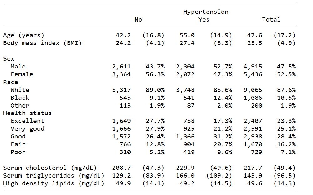
Table of statistical test results
Sometimes, we wish to report a formal hypothesis test for a group of variables. The table below reports the means for a group of continuous variables for participants without hypertension, with hypertension, the difference between the means, and the p-value for a t test.
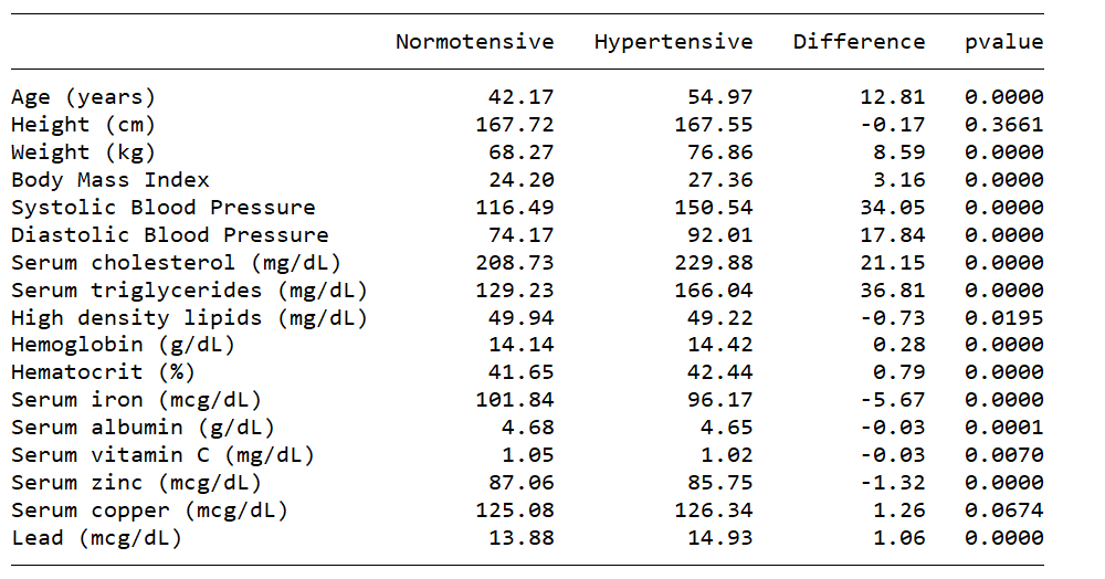
Table for multiple regression models
We may also wish to create a table to compare the results of several regression models. The table below displays the odds ratios and standard errors for the covariates of three logistic regression models along with the AIC and BIC for each model.
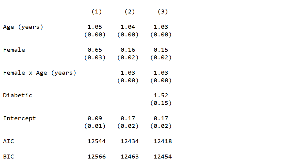
Table for a single regression model
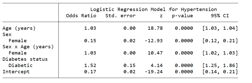
We may also wish to display the results of our final regression model. The table below displays the odds ratio, standard error, z score, p-value, and 95% confidence interval for each covariate in our final model.
You may prefer a different layout for your tables, and that is the point of this series of blog posts. My goal is to show you how to create your own customized tables and import them into your documents.
The data
Let’s begin by typing webuse nhanes2l to open a dataset that contains data from the National Health and Nutrition Examination Survey (NHANES), and let’s describe some of the variables we’ll be using.
. webuse nhanes2l
(Second National Health and Nutrition Examination Survey)

. describe age sex race height weight bmi highbp
>          bpsystol bpdiast tcresult tgresult hdresult

Variable      Storage   Display    Value
    name         type    format    label      Variable label
------------------------------------------------------------------------------------------------------------------------
age             byte    %9.0g                 Age (years)
sex             byte    %9.0g      sex        Sex
race            byte    %9.0g      race       Race
height          float   %9.0g                 Height (cm)
weight          float   %9.0g                 Weight (kg)
bmi             float   %9.0g                 Body mass index (BMI)
highbp          byte    %8.0g               * High blood pressure
bpsystol        int     %9.0g                 Systolic blood pressure
bpdiast         int     %9.0g                 Diastolic blood pressure
tcresult        int     %9.0g                 Serum cholesterol (mg/dL)
tgresult        int     %9.0g                 Serum triglycerides (mg/dL)
hdresult        int     %9.0g                 High density lipids (mg/dL)
This dataset contains demographic, anthropometric, and biological measures for participants in the United States. We will ignore the survey weights for now so that we can focus on the syntax for creating tables.
Introduction to the table command
The basic syntax of table is table (RowVars) (ColVars). The example below creates a table for the row variable highbp.
. table (highbp) ()

--------------------------------
                    |  Frequency
--------------------+-----------
High blood pressure |
  0                 |      5,975
  1                 |      4,376
  Total             |     10,351
--------------------------------
By default, the table displays the frequency for each category of highbp and the total frequency. The second set of empty parentheses in this example is not necessary because there is no column variable.
The example below creates a table for the column variable highbp. The first set of empty parentheses is necessary in this example so that table knows that highbp is a column variable.
. table () (highbp)

------------------------------------
          |    High blood pressure
          |       0       1    Total
----------+-------------------------
Frequency |   5,975   4,376   10,351
------------------------------------
The example below creates a cross-tabulation for the row variable sex and the column variable highbp. The row and column totals are included by default.
. table (sex) (highbp)

-----------------------------------
         |    High blood pressure
         |       0       1    Total
---------+-------------------------
Sex      |
  Male   |   2,611   2,304    4,915
  Female |   3,364   2,072    5,436
  Total  |   5,975   4,376   10,351
-----------------------------------
We can remove the row and column totals by including the nototals option.
. table (sex) (highbp), nototals

---------------------------------
         |   High blood pressure
         |          0           1
---------+-----------------------
Sex      |
  Male   |      2,611       2,304
  Female |      3,364       2,072
---------------------------------
We can also specify multiple row or column variables, or both. The example below displays frequencies for categories of sex nested within categories of highbp.
. table (highbp sex) (), nototals

--------------------------------
                    |  Frequency
--------------------+-----------
High blood pressure |
  0                 |
    Sex             |
      Male          |      2,611
      Female        |      3,364
  1                 |
    Sex             |
      Male          |      2,304
      Female        |      2,072
--------------------------------
Or we can display frequencies for categories of highbp nested within categories of sex as in the example below. The order of the variables in the parentheses determines the nesting structure in the table.
. table (sex highbp) (), nototals

------------------------------------
                        |  Frequency
------------------------+-----------
Sex                     |
  Male                  |
    High blood pressure |
      0                 |      2,611
      1                 |      2,304
  Female                |
    High blood pressure |
      0                 |      3,364
      1                 |      2,072
------------------------------------
We can specify similar nesting structures for multiple column variables. The example below displays frequencies for categories of sex nested within categories of highbp.
. table () (highbp sex), nototals

--------------------------------------------
          |        High blood pressure
          |         0                1
          |        Sex              Sex
          |   Male   Female    Male   Female
----------+---------------------------------
Frequency |  2,611    3,364   2,304    2,072
--------------------------------------------
Or we can display frequencies for categories of highbp nested within categories of sex as in the example below. Again, the order of the variables in the parentheses determines the nesting structure in the table.
. table () (sex highbp), nototals

----------------------------------------------------------
          |                       Sex
          |           Male                   Female
          |   High blood pressure     High blood pressure
          |          0           1           0           1
----------+-----------------------------------------------
Frequency |      2,611       2,304       3,364       2,072
----------------------------------------------------------
You can even specify three, or more, row or column variables. The example below displays frequencies for categories of diabetes nested within categories of sex nested within categories of highbp.
. table (highbp sex diabetes) (), nototals

------------------------------------
                        |  Frequency
------------------------+-----------
High blood pressure     |
  0                     |
    Sex                 |
      Male              |
        Diabetes status |
          Not diabetic  |      2,533
          Diabetic      |         78
      Female            |
        Diabetes status |
          Not diabetic  |      3,262
          Diabetic      |        100
  1                     |
    Sex                 |
      Male              |
        Diabetes status |
          Not diabetic  |      2,165
          Diabetic      |        139
      Female            |
        Diabetes status |
          Not diabetic  |      1,890
          Diabetic      |        182
------------------------------------
The totals() option
We can include totals for a particular row or column variable by including the variable name in the totals() option. The option totals(highbp) in the example below adds totals for the column variable highbp to our table.
. table (sex) (highbp), totals(highbp)

---------------------------------
         |   High blood pressure
         |          0           1
---------+-----------------------
Sex      |
  Male   |      2,611       2,304
  Female |      3,364       2,072
  Total  |      5,975       4,376
---------------------------------
The option totals(sex) in the example below adds totals for the row variable sex to our table.
. table (sex) (highbp), totals(sex)

-----------------------------------
         |    High blood pressure
         |       0        1   Total
---------+-------------------------
Sex      |
  Male   |   2,611    2,304   4,915
  Female |   3,364    2,072   5,436
-----------------------------------
We can also specify row or column variables for a particular variable even when there are multiple row or column variables. The example below displays totals for the row variable highbp, even though there are two row variables in the table.
. table (sex highbp) (), totals(highbp)

------------------------------------
                        |  Frequency
------------------------+-----------
Sex                     |
  Male                  |
    High blood pressure |
      0                 |      2,611
      1                 |      2,304
  Female                |
    High blood pressure |
      0                 |      3,364
      1                 |      2,072
  Total                 |
    High blood pressure |
      0                 |      5,975
      1                 |      4,376
------------------------------------
The statistic() options
Frequencies are displayed by default, but you can specify other statistics with the statistic() option. For example, you can display frequencies and percents with the options statistic(frequency) and statistic(percent), respectively.
. table (sex) (highbp),
>       statistic(frequency)
>       statistic(percent)
>       nototals

--------------------------------------
              |   High blood pressure
              |          0           1
--------------+-----------------------
Sex           |
  Male        |
    Frequency |      2,611       2,304
    Percent   |      25.22       22.26
  Female      |
    Frequency |      3,364       2,072
    Percent   |      32.50       20.02
--------------------------------------
We can also include the mean and standard deviation of age with the options statistic(mean age) and statistic(sd age), respectively.
. // FORMAT THE NUMBERS IN THE OUTPUT
. table (sex) (highbp),
>       statistic(frequency)
>       statistic(percent)
>       statistic(mean age)
>       statistic(sd age)
>       nototals

-----------------------------------------------
                       |   High blood pressure
                       |          0           1
-----------------------+-----------------------
Sex                    |
  Male                 |
    Frequency          |      2,611       2,304
    Percent            |      25.22       22.26
    Mean               |    42.8625    52.59288
    Standard deviation |    16.9688    15.88326
  Female               |
    Frequency          |      3,364       2,072
    Percent            |      32.50       20.02
    Mean               |   41.62366    57.61921
    Standard deviation |   16.59921    13.25577
-----------------------------------------------
You can view a complete list of statistics for the statistic() option in the Stata manual.
The nformat() and sformat() options
We can use the nformat() option to specify the numerical display format for statistics in our table. In the example below, the option nformat(%9.0fc frequency) displays frequency with commas in the thousands place and no digits to the right of the decimal. The option nformat(%6.2f mean sd) displays the mean and standard deviation with two digits to the right of the decimal.
. table (sex) (highbp),
>       statistic(frequency)
>       statistic(percent)
>       statistic(mean age)
>       statistic(sd age)
>       nototals
>       nformat(%9.0fc frequency)
>       nformat(%6.2f  mean sd)

-----------------------------------------------
                       |   High blood pressure
                       |          0           1
-----------------------+-----------------------
Sex                    |
  Male                 |
    Frequency          |      2,611       2,304
    Percent            |      25.22       22.26
    Mean               |      42.86       52.59
    Standard deviation |      16.97       15.88
  Female               |
    Frequency          |      3,364       2,072
    Percent            |      32.50       20.02
    Mean               |      41.62       57.62
    Standard deviation |      16.60       13.26
-----------------------------------------------
We can use the sformat() option to add strings to the statistics in our table. In the example below, the option sformat(“%s%%” percent) adds “%” to the statistic percent, and the option sformat(“(%s)” sd) places parentheses around the standard deviation.
. table (sex) (highbp),
>       statistic(frequency)
>       statistic(percent)
>       statistic(mean age)
>       statistic(sd age)
>       nototals
>       nformat(%9.0fc frequency)
>       nformat(%6.2f  mean sd)
>       sformat("%s%%" percent)
>       sformat("(%s)" sd)

-----------------------------------------------
                       |   High blood pressure
                       |          0           1
-----------------------+-----------------------
Sex                    |
  Male                 |
    Frequency          |      2,611       2,304
    Percent            |     25.22%      22.26%
    Mean               |      42.86       52.59
    Standard deviation |    (16.97)     (15.88)
  Female               |
    Frequency          |      3,364       2,072
    Percent            |     32.50%      20.02%
    Mean               |      41.62       57.62
    Standard deviation |    (16.60)     (13.26)
-----------------------------------------------
The style() option
We can use the style() option to apply a predefined style to a table. In the example below, the option style(table-1) applies Stata’s predefined style table-1 to our table. This style changed the appearance of the row labels. You can view a complete list of Stata’s predefined styles in the manual, and I will show you how to create your own styles in a future blog post.
. table (sex) (highbp),
>       statistic(frequency)
>       statistic(percent)
>       statistic(mean age)
>       statistic(sd age)
>       nototals
>       nformat(%9.0fc frequency)
>       nformat(%6.2f  mean sd)
>       sformat("%s%%" percent)
>       sformat("(%s)" sd)
>       style(table-1)

---------------------------------
         |   High blood pressure
         |          0           1
---------+-----------------------
     Sex |
  Male   |      2,611       2,304
         |     25.22%      22.26%
         |      42.86       52.59
         |    (16.97)     (15.88)
         |
Female   |      3,364       2,072
         |     32.50%      20.02%
         |      41.62       57.62
         |    (16.60)     (13.26)
---------------------------------
Conclusion
We learned a lot about the new-and-improved table command, but we have barely scratched the surface. We have learned how to create tables and use the nototals, totals(), statistic(), nformat(), sformat(), and style() options. There are many other options, and you can read about them in the manual. I’ll show you how to use collect to customize the appearance of your tables in my next post.
You can also visit the Stata YouTube Channel to learn how to create tables using the table dialog box and the Tables Builder.
Customizable tables in Stata 17
Customizable tables in Stata 17: Cross-tabulations
Customizable tables in Stata 17: One-way tables of summary
Customizable tables in Stata 17: Two-way tables of summary statistics
Customizable tables in Stata 17: How to create tables for a regression model
Customizable tables in Stata 17: How to create tables for multiple regression models