Customizable tables in Stata 17, part 2: The new collect command
In my last post, I showed you how to use the new-and-improved table command to create a table and how to use some of the options to customize the table. In this post I want to introduce the collect commands. Many Stata commands begin with collect, and they can be used to create collections, customize table layouts, format the numbers in the tables, and export tables to documents. There are so many new collect commands that we created a new Customizable Tables and Collected Results Reference Manual. Today, I want to show you how to use some of the collect commands to customize the look of your tables. I will show you more advanced uses of collect in future posts.
We left off with the table below near the end of my last post. We used the style() option to format our table using one of Stata’s predefined styles. I have omitted the style() option in the table below so that we can use a series of collect commands to customize the table ourselves.
. table (sex) (highbp),
>       statistic(frequency)
>       statistic(percent)
>       statistic(mean age)
>       statistic(sd age)
>       nototals
>       nformat(%9.0fc frequency)
>       sformat("%s%%" percent)
>       nformat(%6.2f  mean sd)
>       sformat("(%s)" sd)

-----------------------------------------------
                       |   High blood pressure
                       |          0           1
-----------------------+-----------------------
Sex                    |
  Male                 |
    Frequency          |      2,611       2,304
    Percent            |     25.22%      22.26%
    Mean               |      42.86       52.59
    Standard deviation |    (16.97)     (15.88)
  Female               |
    Frequency          |      3,364       2,072
    Percent            |     32.50%      20.02%
    Mean               |      41.62       57.62
    Standard deviation |    (16.60)     (13.26)
-----------------------------------------------
Collections, dimensions, and levels
The table command above automatically created a collection for us. Collections contain “dimensions”, and we can view the dimensions in our collection by typing collect dims.
. collect dims

Collection dimensions
Collection: Table
-----------------------------------------
                   Dimension   No. levels
-----------------------------------------
Layout, style, header, label
                      across   2
                      cmdset   1
                     colname   1
                     command   1
                      highbp   2
                      result   4
                         sex   2
                     statcmd   4
                         var   2

Style only
                border_block   4
                   cell_type   4
-----------------------------------------
The output tells us that our collection is named Table. Our collection includes dimensions with names such as across, colname, command, and others. The output also tells us the number of levels of each dimension.
Our collection also includes the dimensions sex and highbp, which are created from our row and column variables. We can view the levels of sex by typing collect levelsof sex.
. collect levelsof sex

Collection: Table
 Dimension: sex
    Levels: 1 2
The output tells us that the dimension sex has levels 1 and 2. Levels can have labels, and we can view the labels of the dimension sex by typing collect label list sex.
. collect label list sex, all

  Collection: Table
   Dimension: sex
       Label: Sex
Level labels:
          .m  Total
           1  Male
           2  Female
The output tells us that level 1 is labeled “Male” and level 2 is labeled “Female”. The option all in the collect label list command shows us that there is an additional level named .m that is labeled “Total”.
We can view the levels of the dimension highbp by typing collect levelsof highbp.
. collect levelsof highbp

Collection: Table
 Dimension: highbp
    Levels: 0 1
The dimension highbp has levels 0 and 1. We can view the level labels by typing collect label list highbp.
. collect label list highbp, all

  Collection: Table
   Dimension: highbp
       Label: High blood pressure
Level labels:
          .m  Total
           0
           1
The output tells us that the level .m is labeled “Total”, but the levels 0 and 1 do not have labels. We can add labels to the levels by typing collect label levels highbp and assigning labels to each level.
. collect label levels highbp 0 "No" 1 "Yes"

. collect label list highbp, all

  Collection: Table
   Dimension: highbp
       Label: High blood pressure
Level labels:
          .m  Total
           0  No
           1  Yes
Let’s type collect preview to view the changes to our table.
. collect preview

-----------------------------------------------
                       |   High blood pressure
                       |         No         Yes
-----------------------+-----------------------
Sex                    |
  Male                 |
    Frequency          |      2,611       2,304
    Percent            |     25.22%      22.26%
    Mean               |      42.86       52.59
    Standard deviation |    (16.97)     (15.88)
  Female               |
    Frequency          |      3,364       2,072
    Percent            |     32.50%      20.02%
    Mean               |      41.62       57.62
    Standard deviation |    (16.60)     (13.26)
-----------------------------------------------
The table now displays the labels “No” and “Yes” for the levels of highbp. The output and the table above also tell us that the dimension highbp is labeled “High blood pressure”. Dimensions created from variables are automatically labeled with the variable label. We can change the label for the dimension highbp by typing collect label dim highbp and then specifying a new label.
. collect label dim highbp "Hypertension", modify
We can preview the change in our table by typing collect preview.
. collect preview

-------------------------------------------
                       |     Hypertension
                       |       No       Yes
-----------------------+-------------------
Sex                    |
  Male                 |
    Frequency          |    2,611     2,304
    Percent            |   25.22%    22.26%
    Mean               |    42.86     52.59
    Standard deviation |  (16.97)   (15.88)
  Female               |
    Frequency          |    3,364     2,072
    Percent            |   32.50%    20.02%
    Mean               |    41.62     57.62
    Standard deviation |  (16.60)   (13.26)
-------------------------------------------
Or we can type collect label list highbp to verify that we have changed the dimension label to “Hypertension”.
. collect label list highbp, all

  Collection: Table
   Dimension: highbp
       Label: Hypertension
Level labels:
          .m  Total
           0  No
           1  Yes
Note that we did not change the variable label for the variable highbp. We changed the label for the dimension highbp. This may seem confusing at first, so let’s review the logic of collections.
Datasets contain variables and variables can have categories. Collections, dimensions, and levels are similar concepts that are used to create custom tables. A collection is analogous to a dataset. A dimension is analogous to a variable. And a level is analogous to a category of a categorical variable. Dimensions can have labels just like variables. Levels can have labels just like the value labels of the categories of a variable.
I can think of at least two advantages of using collections to label elements of collections. First, collections allow us to specify custom labels for a particular table without altering our original data. We could simply change the variable labels and value labels of our variables to change the labels in our tables. But often we wish to change the labels for some tables and not others. And we may wish to use different labels for our graphs. Second, collections allow us to create and label dimensions that are not based on variables in our dataset. Recall that there were other dimensions in the output when we typed collect dims.
. collect dims

Collection dimensions
Collection: Table
-----------------------------------------
                   Dimension   No. levels
-----------------------------------------
Layout, style, header, label
                      across   2
                      cmdset   1
                     colname   1
                     command   1
                      highbp   2
                      result   4
                         sex   2
                     statcmd   4
                         var   2

Style only
                border_block   4
                   cell_type   4
-----------------------------------------
The output tells us that there is a dimension named result that has four levels. Let’s type collect label list result to learn more about the dimension result.
. collect label list result, all

  Collection: Table
   Dimension: result
       Label: Result
Level labels:
   frequency  Frequency
        mean  Mean
     percent  Percent
          sd  Standard deviation
The output tells us that the dimension result is part of the Table collection and has levels named frequency, mean, percent, and sd. These levels are labeled “Frequency”, “Mean”, “Percent”, and “Standard deviation”, respectively.
Note that the dimension result is not based on a variable in our dataset. It was created by the statistic() options in our table command above.
We can type collect label levels to modify the level labels for the dimension result
. collect label levels result frequency "Freq."
>                             mean      "Mean (Age)"
>                             percent   "Percent"
>                             sd         "SD (Age)"
>                             , modify

. collect preview

-----------------------------------
               |     Hypertension
               |       No       Yes
---------------+-------------------
Sex            |
  Male         |
    Freq.      |    2,611     2,304
    Percent    |   25.22%    22.26%
    Mean (Age) |    42.86     52.59
    SD (Age)   |  (16.97)   (15.88)
  Female       |
    Freq.      |    3,364     2,072
    Percent    |   32.50%    20.02%
    Mean (Age) |    41.62     57.62
    SD (Age)   |  (16.60)   (13.26)
-----------------------------------
Using collect to customize the appearance of tables
There are many collect commands that we can use to customize the appearance of our table. For example, the vertical line in our table is a border on the right side of the first column. We can remove the border using collect style cell.
. collect style cell border_block, border(right, pattern(nil))

. collect preview

---------------------------------
                   Hypertension
                     No       Yes
---------------------------------
Sex
  Male
    Freq.         2,611     2,304
    Percent      25.22%    22.26%
    Mean (Age)    42.86     52.59
    SD (Age)    (16.97)   (15.88)
  Female
    Freq.         3,364     2,072
    Percent      32.50%    20.02%
    Mean (Age)    41.62     57.62
    SD (Age)    (16.60)   (13.26)
---------------------------------
There are many collect style commands, including collect style cell, collect style row, collect style column, and collect style header. We can use these commands to customize the borders, shading, fonts, colors, and other attributes of our tables. We will explore these in more detail in future blog posts.
Saving labels and styles
Once we like the look of our table, we can type collect label save to save our custom labels, and we can type collect style save to save our custom style.
. collect label save MyLabels, replace
(labels from Table saved to file MyLabels.stjson)

. collect style save MyStyle, replace
(style from Table saved to file MyStyle.stjson)
Then, we can apply our labels and style to future tables using the style() and label() options in our table commands.
. table (sex) (highbp),
>       statistic(frequency)
>       statistic(percent)
>       statistic(mean age)
>       statistic(sd age)
>       nototals
>       nformat(%9.0fc frequency)
>       sformat("%s%%" percent)
>       nformat(%6.2f  mean sd)
>       sformat("(%s)" sd)
>       style(MyStyle, override)
>       label(MyLabels)

---------------------------------
                   Hypertension
                     No       Yes
---------------------------------
Sex
  Male
    Freq.         2,611     2,304
    Percent      25.22%    22.26%
    Mean (Age)    42.86     52.59
    SD (Age)    (16.97)   (15.88)
  Female
    Freq.         3,364     2,072
    Percent      32.50%    20.02%
    Mean (Age)    41.62     57.62
    SD (Age)    (16.60)   (13.26)
---------------------------------
Exporting tables to documents with collect export
We can use collect export to export our table to many different file formats, including Microsoft Word and Excel, HTML 5 with CSS files, Markdown, PDF, LaTeX, SMCL, and plain text.
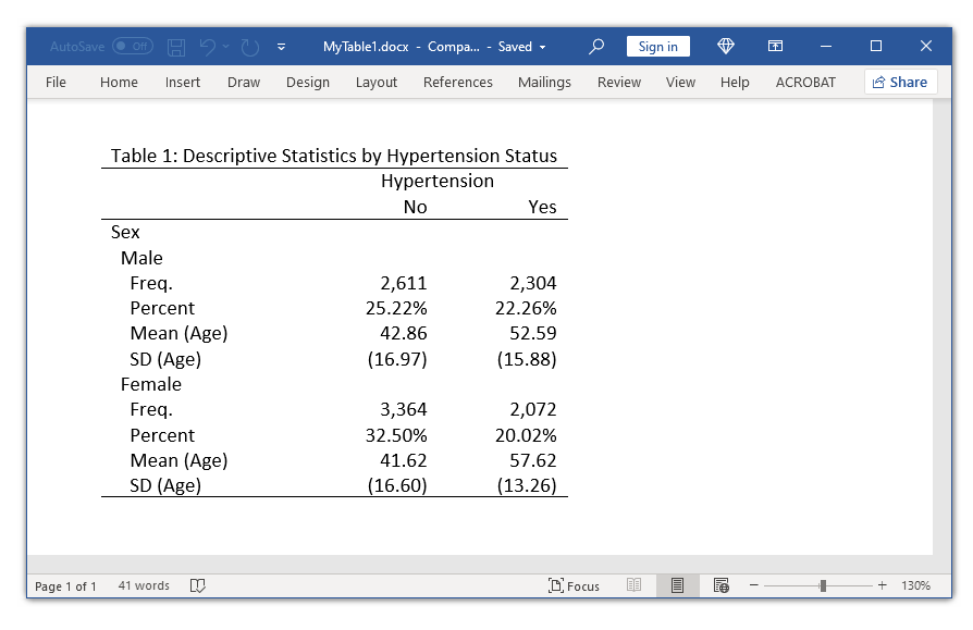
I have used collect style putdocx in the example below to add a title to our table and to automatically fit the table within a Microsoft Word document. Then, I have used collect export to export the table to a Microsoft Word document.
. collect style putdocx, layout(autofitcontents)
>         title("Table 1: Descriptive Statistics by Hypertension Status")

. collect export MyTable1.docx, as(docx) replace
(collection Table exported to file MyTable1.docx)
Exporting tables to documents with putdocx collect
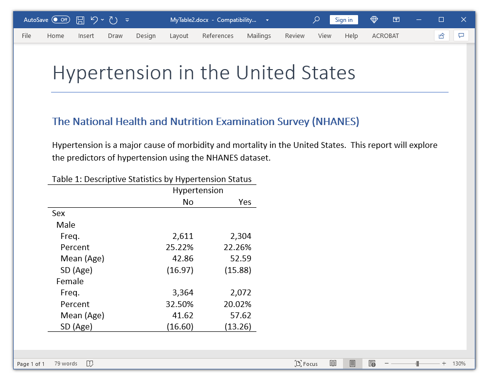
Stata’s putdocx command is a powerful tool for creating sophisticated Microsoft Word documents that include text, tables, and graphs. We can also export our tables to these documents using putdocx collect. I have used a red font in the code block below to show you how to export our table to a Microsoft Word document using putdocx collect.
putdocx begin

putdocx paragraph, style(Title)

putdocx text ("Hypertension in the United States")

putdocx paragraph, style(Heading1)

putdocx text ("The National Health and Nutrition Examination Survey (NHANES)")

putdocx paragraph

putdocx text ("Hypertension is a major cause of morbidity and mortality in ")

putdocx text ("the United States.  This report will explore the predictors ")

putdocx text ("of hypertension using the NHANES dataset.")

collect style putdocx, layout(autofitcontents)                          ///

title("Table 1: Descriptive Statistics by Hypertension Status")

putdocx collect

putdocx save MyTable2.docx, replace
Conclusion
We learned a lot about the collect commands, but we have barely scratched the surface. We learned about collections, dimensions, and levels. We learned how to create and modify the labels of dimensions and their labels; how to use collect style to customize the style of our tables; how to save our labels and styles and apply them to future tables; and how to export our tables to documents.
In future blog posts, I will show you how to use table and collect to re-create the examples I showed you at the beginning of my last post.
You can also visit the Stata YouTube Channel to learn how to create tables using the table dialog box and the Tables Builder.
Customizable tables in Stata 17
Customizable tables in Stata 17: Cross-tabulations
Customizable tables in Stata 17: One-way tables of summary
Customizable tables in Stata 17: Two-way tables of summary statistics
Customizable tables in Stata 17: How to create tables for a regression model
Customizable tables in Stata 17: How to create tables for multiple regression models