Customizable tables in Stata 17, part 7: Saving and using custom styles and labels
In Customizable tables in Stata 17, part 5, I showed you how to use the new and improved table command to create a table of results from a logistic regression model. We are likely to create many more tables of regression results, and we will probably use the same style and labels. In this post, I will show you how to save your styles and labels so that you can use them to format future tables. I will use the Microsoft Word document that we created in part 5 as our goal.
Create the basic table
Let’s begin by typing webuse nhanes2l to open the NHANES dataset. Then we will use table to create a basic table for a logistic regression model for the binary outcome highbp. The table includes the odds ratios, standard errors, z statistics, p-values, and confidence intervals. Note that I have used Stata’s factor-variable notation in the example below to include the main effect of the continuous variable age, the main effects of the categorical variables sex and diabetes, and the interaction of age and sex.
. webuse nhanes2l
(Second National Health and Nutrition Examination Survey)

. table () (command result),
>           command(_r_b _r_se _r_z _r_p _r_ci
>                   : logistic highbp c.age##i.sex i.diabetes)

--------------------------------------------------------------------------------------------------
                             |                logistic highbp c.age##i.sex i.diabetes
                             |  Coefficient   Std. error        z   p-value          95% CI
-----------------------------+--------------------------------------------------------------------
Age (years)                  |     1.034281     .0018566    18.78     0.000   1.030648    1.037926
Sex=Male                     |            1            0
Sex=Female                   |     .1549363     .0223461   -12.93     0.000   .1167849    .2055511
Sex=Male # Age (years)       |            1            0
Sex=Female # Age (years)     |     1.028856     .0027958    10.47     0.000   1.023391    1.034351
Diabetes status=Not diabetic |            1            0
Diabetes status=Diabetic     |     1.521011      .154103     4.14     0.000   1.247073    1.855124
Intercept                    |     .1730928     .0157789   -19.24     0.000    .144772    .2069537
--------------------------------------------------------------------------------------------------
Create and save a custom style
Let’s type collect clear to clear any collections from Stata’s memory.
. collect clear
Then we can use the same collect style commands that we used to format our table in part 5. I have included comments in the code block below to remind us of the purpose of each line.
// TURN OFF BASE LEVELS FOR FACTOR VARIABLES
collect style showbase off
// STACK THE ROW LEVEL LABELS AND CHANGE THE INTERACTION DELIMITER
collect style row stack, delimiter(" x ") nobinder
// REMOVE THE VERTICAL LINE
collect style cell border_block, border(right, pattern(nil))
// FORMAT THE NUMBERS
collect style cell result[_r_b _r_se _r_ci], nformat(%8.2f)
collect style cell result[_r_p], nformat(%5.4f)
collect style cell result[_r_ci], sformat("[%s]") cidelimiter(,)
// HIDE THE LOGISTIC REGRESSION COMMAND
collect style header command, level(hide)
Finally, we can type collect style save to save this style to a file named MyLogitStyle.stjson.
. collect style save MyLogitStyle, replace
(style from mylogit saved to file MyLogitStyle.stjson)
Create and save level labels
We can also save custom level labels. The coefficients in our logistic regression output are actually odds ratios. In part 5, we used collect label levels to change the label for the level _r_b in the dimension result from “Coefficient” to “Odds Ratio”.
collect label levels result _r_b "Odds Ratio", modify
We can use collect label save to save our custom level label to a file named MyLogitLabels.stjson.
. collect label save MyLogitLabels, replace
(labels from mylogit saved to file MyLogitLabels.stjson)
Using our saved styles and labels
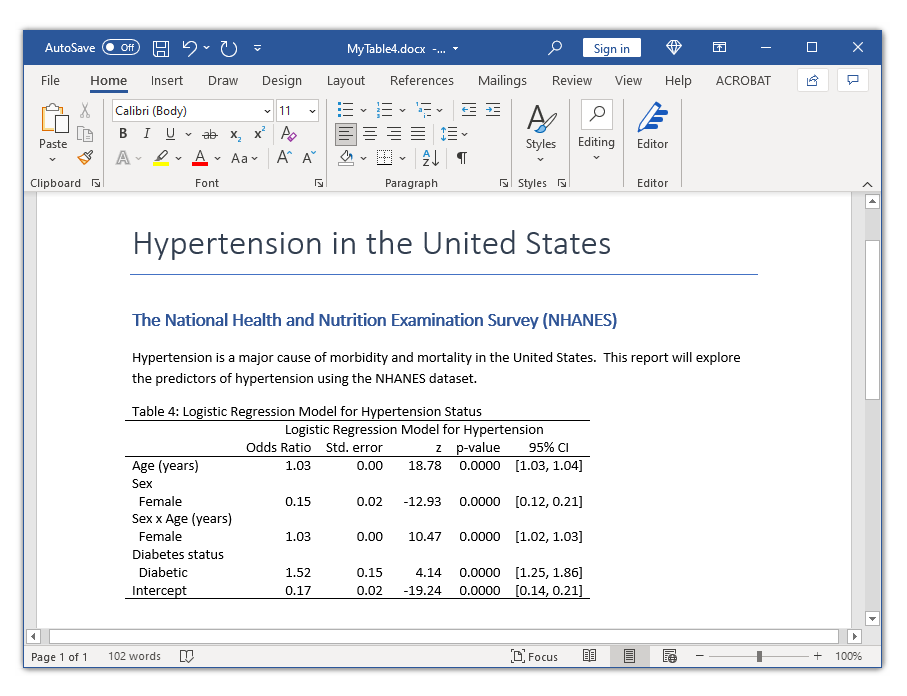
We can apply our style and labels to a table using the style() and label() options when we define our table. If you are in the same directory where you just saved the labels and styles, you can refer to them simply by their names. However, if you are in a different directory you can specify the full path.
. table () (command result),
>          command(_r_b _r_se _r_z _r_p _r_ci
>                  : logistic highbp c.age##i.sex i.diabetes)
>          style(c:\MyFolder\MyLogitStyle.stjson, override)
>          label(c:\MyFolder\MyLogitLabels.stjson)

-------------------------------------------------------------------------------
                   Odds Ratio   Std. error        z   p-value        95% CI
-------------------------------------------------------------------------------
Age (years)              1.03         0.00    18.78    0.0000   [1.03,    1.04]
Sex
  Female                 0.15         0.02   -12.93    0.0000   [0.12,    0.21]
Sex x Age (years)
  Female                 1.03         0.00    10.47    0.0000   [1.02,    1.03]
Diabetes status
  Diabetic               1.52         0.15     4.14    0.0000   [1.25,    1.86]
Intercept                0.17         0.02   -19.24    0.0000   [0.14,    0.21]
-------------------------------------------------------------------------------
Or, even better, we can save our styles and labels where we can use them anytime. We can make our styles and labels automatically available by storing the files in our personal ado-directory. You can type sysdir to locate your personal ado-directory.
. sysdir
   STATA:  C:\Program Files\Stata17\
    BASE:  C:\Program Files\Stata17\ado\base\
    SITE:  C:\Program Files\Stata17\ado\site\
    PLUS:  C:\Users\ChuckStata\ado\plus\
PERSONAL:  c:\ado\personal\
OLDPLACE:  c:\ado\
My personal ado-directory is c:\ado\personal\, so I will save my style and label files in that folder.
. collect style save "c:\ado\personal\MyLogitStyle", replace
(style from mylogit saved to file c:\ado\personal\MyLogitStyle.stjson)

. collect label save "c:\ado\personal\MyLogitLabels", replace
(labels from mylogit saved to file c:\ado\personal\MyLogitLabels.stjson)
Now I can use MyLogitStyle and MyLogitLabels anytime to format other tables.
Using our saved styles and labels with other tables
Let’s clear Stata’s memory and use the Hosmer and Lemeshow low birthweight dataset. We are interested in predictors of low infant birthweight (low), defined as birthweight less than 2,500 grams.
. webuse lbw, clear
(Hosmer & Lemeshow data)

. describe low age smoke ht

Variable      Storage   Display    Value
    name         type    format    label      Variable label
------------------------------------------------------------------------------------------------------------------------
low             byte    %8.0g                 Birthweight<2500g
age             byte    %8.0g                 Age of mother
smoke           byte    %9.0g      smoke      Smoked during pregnancy
ht              byte    %8.0g                 Has history of hypertension
Next let’s create a table for the output of a logistic regression command for the binary dependent variable low. We can format our table using MyLogitStyle and MyLogitLabels.
. table () (command result),
>          command(_r_b _r_se _r_z _r_p _r_ci
>                  : logistic low c.age##i.smoke ht)
>          style(MyLogitStyle, override)
>          label(MyLogitLabels)

----------------------------------------------------------------------------------------------------
                                         Odds Ratio   Std. error       z   p-value        95% CI
----------------------------------------------------------------------------------------------------
Age of mother                                  0.92         0.04   -1.85    0.0646   [0.84,    1.01]
Smoked during pregnancy
  Smoker                                       0.36         0.56   -0.66    0.5082   [0.02,    7.37]
Smoked during pregnancy x Age of mother
  Smoker                                       1.08         0.07    1.14    0.2542   [0.95,    1.23]
Has history of hypertension                    3.47         2.15    2.00    0.0456   [1.02,   11.72]
Intercept                                      2.16         2.27    0.73    0.4642   [0.28,   16.90]
----------------------------------------------------------------------------------------------------
The overall format of our table looks like we expected. But the variable labels are too long for our table.
The row labels in our table are stored in the dimension colname. We can type collect label list to view the level labels.
. collect label list colname, all

  Collection: Table
   Dimension: colname
       Label: Covariate names and column names
Level labels:
       _cons  Intercept
       _hide
         age  Age of mother
          c1
          c2
          c3
          c4
          ht  Has history of hypertension
       smoke  Smoked during pregnancy
Let’s use collect label levels to modify the labels of the levels age, ht, and smoke.
. collect label levels colname age "Age", modify

. collect label levels colname ht "Hypertension", modify

. collect label levels colname smoke "Smoke", modify
Now we can type collect preview to check our work.
. collect preview

-------------------------------------------------------------------------
              Odds Ratio   Std. error       z   p-value        95% CI
-------------------------------------------------------------------------
Age                 0.92         0.04   -1.85    0.0646   [0.84,    1.01]
Smoke
  Smoker            0.36         0.56   -0.66    0.5082   [0.02,    7.37]
Smoke x Age
  Smoker            1.08         0.07    1.14    0.2542   [0.95,    1.23]
Hypertension        3.47         2.15    2.00    0.0456   [1.02,   11.72]
Intercept           2.16         2.27    0.73    0.4642   [0.28,   16.90]
-------------------------------------------------------------------------
Note that we still used collect to customize our table, even though we did most of the work with our saved styles and labels.
Conclusion
In this post, we learned how to use collect style save and collect label save to save our custom styles and labels. We also learned how to apply those custom styles and labels to other tables. Stata has many predefined styles, and you can learn more about them in the manual.
The ability to save and reuse custom styles and labels allows us to streamline and automate our workflow for creating documents. For example, many people in academic settings submit manuscripts for publication in academic journals. They can create custom formats and labels that meet each journal’s requirements and apply them to their manuscripts. People in business or government settings may report the same information to different organizations, and they can save custom styles and labels for each report. Investing the time to create custom styles and layouts will pay dividends in saved time later.
This is the final post I had planned for the “Customizable tables in Stata 17” series. My goal was to explain the basics of the new table and collect commands, show you a few useful examples, and demonstrate how you can use these tools to create your own custom tables. I hope I’ve accomplished that goal, and I’ve had so much fun that I would not rule out future posts on this topic!