Customizable tables in Stata 17, part 5: Tables for one regression model
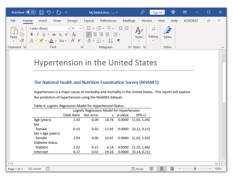
In my last post, I showed you how to use the new and improved table command with the command() option to create a table of statistical tests. In this post, I want to show you how to use the command() option to create a table for a single regression model. Our goal is to create the table in the Microsoft Word document below.
Create the basic table
Let’s begin by typing webuse nhanes2l to open the NHANES dataset, and let’s type describe to examine some of the variables.
. webuse nhanes2l
(Second National Health and Nutrition Examination Survey)

. describe highbp age sex diabetes

Variable      Storage   Display    Value
    name         type    format    label      Variable label
-------------------------------------------------------------------------------
highbp          byte    %8.0g               * High blood pressure
age             byte    %9.0g                 Age (years)
sex             byte    %9.0g      sex        Sex
diabetes        byte    %12.0g     diabetes   Diabetes status
The dataset includes age, sex, an indicator for high blood pressure (highbp), and an indicator for diabetes (diabetes). We would like to fit a logistic regression model for the binary outcome highbp and create a table of the odds ratios, standard errors, z statistics, p-values, and confidence intervals. Note that I have used Stata’s factor-variable notation in the example below to include the main effect of the continuous variable age, the main effect of the categorical variables sex and diabetes, and the interaction of age and sex.
. logistic highbp c.age##i.sex i.diabetes

Logistic regression                                    Number of obs =  10,349
                                                       LR chi2(4)    = 1691.59
                                                       Prob > chi2   =  0.0000
Log likelihood = -6203.8722                            Pseudo R2     =  0.1200

------------------------------------------------------------------------------
      highbp | Odds ratio   Std. err.      z    P>|z|     [95% conf. interval]
-------------+----------------------------------------------------------------
         age |   1.034281   .0018566    18.78   0.000     1.030648    1.037926
             |
         sex |
     Female  |   .1549363   .0223461   -12.93   0.000     .1167849    .2055511
             |
   sex#c.age |
     Female  |   1.028856   .0027958    10.47   0.000     1.023391    1.034351
             |
    diabetes |
   Diabetic  |   1.521011    .154103     4.14   0.000     1.247073    1.855124
       _cons |   .1730928   .0157789   -19.24   0.000      .144772    .2069537
------------------------------------------------------------------------------
Note: _cons estimates baseline odds.
Let’s begin by placing the logistic regression command in the command() option of a table command. There are no row dimensions, and the column dimensions are command and result.
. table () (command result),
>          command(logistic highbp c.age##i.sex i.diabetes)

-----------------------------------------------------------------------
                             |  logistic highbp c.age##i.sex i.diabetes
-----------------------------+-----------------------------------------
Age (years)                  |                                 1.034281
Sex=Male                     |                                        1
Sex=Female                   |                                 .1549363
Sex=Male # Age (years)       |                                        1
Sex=Female # Age (years)     |                                 1.028856
Diabetes status=Not diabetic |                                        1
Diabetes status=Diabetic     |                                 1.521011
Intercept                    |                                 .1730928
-----------------------------------------------------------------------
By default, the table displays the coefficients, which are actually odds ratios because we used the logistic command.
table automatically created a collection named Table, and we can view the dimensions by typing collect dims.
. collect dims

Collection dimensions
Collection: Table
-----------------------------------------
                   Dimension   No. levels
-----------------------------------------
Layout, style, header, label
                      cmdset   1
                       coleq   2
                     colname   13
           colname_remainder   2
                     command   1
                    diabetes   2
               program_class   1
                      result   43
                 result_type   3
                       roweq   1
                     rowname   2
                         sex   2
                     statcmd   1

Style only
                border_block   4
                   cell_type   4
-----------------------------------------
The dimension result has 43 levels. Let’s type collect label list to view the levels and their labels.
. collect label list result, all

  Collection: Table
   Dimension: result
       Label: Result
Level labels:
           N  Number of observations
       N_cdf  Number of completely determined failures
       N_cds  Number of completely determined successes
        _r_b  Coefficient
       _r_ci  __LEVEL__% CI
       _r_df  df
       _r_lb  __LEVEL__% lower bound
        _r_p  p-value
       _r_se  Std. error
       _r_ub  __LEVEL__% upper bound
        _r_z  z
       (output omitted)
We are interested in the levels that begin with _r, so I have omitted much of the output. The levels that begin with _r are the contents of the table of coefficients. For example, the level _r_b contains coefficients (that is, odds ratios), the level _r_se contains the standard errors, and so forth. Note that the confidence interval is stored in a single level, _r_ci, and also in separate levels for the upper and lower bounds, _r_lb and r_ub, respectively.
Let’s add the odds ratio, standard error, and confidence interval to our table by including _r_b _r_se _r_ci to our command() option. We will add the z test and p-value later.
. table () (command result),
>          command(_r_b _r_se _r_ci
>                  : logistic highbp c.age##i.sex i.diabetes)

-------------------------------------------------------------------------------
                             |      logistic highbp c.age##i.sex i.diabetes
                             |  Coefficient   Std. error          95% CI
-----------------------------+-------------------------------------------------
Age (years)                  |     1.034281     .0018566   1.030648    1.037926
Sex=Male                     |            1            0
Sex=Female                   |     .1549363     .0223461   .1167849    .2055511
Sex=Male # Age (years)       |            1            0
Sex=Female # Age (years)     |     1.028856     .0027958   1.023391    1.034351
Diabetes status=Not diabetic |            1            0
Diabetes status=Diabetic     |     1.521011      .154103   1.247073    1.855124
Intercept                    |     .1730928     .0157789    .144772    .2069537
-------------------------------------------------------------------------------
Next let’s customize the display of the numbers in our table. I’ve used nformat() to display the odds ratios, standard errors, and condidence interval with two digits to the right of the decimal. I’ve used sformat() to place square brackets around the confidence interval, and I’ve used cidelimiter() to place a comma between the lower and upper bounds of the confidence interval.
. table () (command result),
>          command(_r_b _r_se _r_ci
>                  : logistic highbp c.age##i.sex i.diabetes)
>          nformat(%5.2f  _r_b _r_se _r_ci )
>          sformat("[%s]"  _r_ci )
>          cidelimiter(,)

---------------------------------------------------------------------------
                             |    logistic highbp c.age##i.sex i.diabetes
                             |    Coefficient    Std. error       95% CI
-----------------------------+---------------------------------------------
Age (years)                  |           1.03          0.00    [1.03, 1.04]
Sex=Male                     |           1.00          0.00
Sex=Female                   |           0.15          0.02    [0.12, 0.21]
Sex=Male # Age (years)       |           1.00          0.00
Sex=Female # Age (years)     |           1.03          0.00    [1.02, 1.03]
Diabetes status=Not diabetic |           1.00          0.00
Diabetes status=Diabetic     |           1.52          0.15    [1.25, 1.86]
Intercept                    |           0.17          0.02    [0.14, 0.21]
---------------------------------------------------------------------------
The column of odds ratios is labeled Coefficient, and we can change it to Odds Ratio using collect label levels.
. collect label levels result _r_b "Odds Ratio", modify

. collect preview

---------------------------------------------------------------------------
                             |    logistic highbp c.age##i.sex i.diabetes
                             |    Odds Ratio     Std. error       95% CI
-----------------------------+---------------------------------------------
Age (years)                  |          1.03           0.00    [1.03, 1.04]
Sex=Male                     |          1.00           0.00
Sex=Female                   |          0.15           0.02    [0.12, 0.21]
Sex=Male # Age (years)       |          1.00           0.00
Sex=Female # Age (years)     |          1.03           0.00    [1.02, 1.03]
Diabetes status=Not diabetic |          1.00           0.00
Diabetes status=Diabetic     |          1.52           0.15    [1.25, 1.86]
Intercept                    |          0.17           0.02    [0.14, 0.21]
---------------------------------------------------------------------------
The dimension command has one level that is labeled with our logistic regression command. We can also modify its label using collect label levels.
. collect label levels command 1
>          "Logistic Regression Model for Hypertension", modify

. collect preview

------------------------------------------------------------------------------
                             |    Logistic Regression Model for Hypertension
                             |     Odds Ratio      Std. error       95% CI
-----------------------------+------------------------------------------------
Age (years)                  |           1.03            0.00     [1.03, 1.04]
Sex=Male                     |           1.00            0.00
Sex=Female                   |           0.15            0.02     [0.12, 0.21]
Sex=Male # Age (years)       |           1.00            0.00
Sex=Female # Age (years)     |           1.03            0.00     [1.02, 1.03]
Diabetes status=Not diabetic |           1.00            0.00
Diabetes status=Diabetic     |           1.52            0.15     [1.25, 1.86]
Intercept                    |           0.17            0.02     [0.14, 0.21]
------------------------------------------------------------------------------
By default, table displays the base level, also known as the ‘referent category’ or ‘referent group’, of factor variables. For example, the row labeled Sex=Male is the base level for the factor variable i.sex. The category Male is used in the denominator of the odds ratio. We can hide the base levels of all factor variables, including interactions, by typing collect style showbase off.
. collect style showbase off

. collect preview

--------------------------------------------------------------------------
                         |    Logistic Regression Model for Hypertension
                         |     Odds Ratio      Std. error       95% CI
-------------------------+------------------------------------------------
Age (years)              |           1.03            0.00     [1.03, 1.04]
Sex=Female               |           0.15            0.02     [0.12, 0.21]
Sex=Female # Age (years) |           1.03            0.00     [1.02, 1.03]
Diabetes status=Diabetic |           1.52            0.15     [1.25, 1.86]
Intercept                |           0.17            0.02     [0.14, 0.21]
--------------------------------------------------------------------------
Next let’s use collect style row to customize the row labels. By default, the variables and categories are displayed side by side with a “binder” character. For example, Sex=Female displays the variable Sex followed by the binder = followed by the category Female. The option stack displays the variable name once and then displays each category below the variable name. The option nobinder removes the binder character, =. Interactions are displayed using the # character and we can use the delimiter(” x “) option to change the interaction delimiter to x.
. collect style row stack, nobinder delimiter(" x ")

. collect preview

-------------------------------------------------------------------
                  |    Logistic Regression Model for Hypertension
                  |     Odds Ratio      Std. error       95% CI
------------------+------------------------------------------------
Age (years)       |           1.03            0.00     [1.03, 1.04]
Sex               |
  Female          |           0.15            0.02     [0.12, 0.21]
Sex x Age (years) |
  Female          |           1.03            0.00     [1.02, 1.03]
Diabetes status   |
  Diabetic        |           1.52            0.15     [1.25, 1.86]
Intercept         |           0.17            0.02     [0.14, 0.21]
-------------------------------------------------------------------
We removed the vertical line from the tables in my previous posts, and we can do the same thing here using collect style cell to remove the right border from the first column.
. collect style cell border_block, border(right, pattern(nil))

. collect preview

-----------------------------------------------------------------
                     Logistic Regression Model for Hypertension
                      Odds Ratio      Std. error       95% CI
-----------------------------------------------------------------
Age (years)                 1.03            0.00     [1.03, 1.04]
Sex
  Female                    0.15            0.02     [0.12, 0.21]
Sex x Age (years)
  Female                    1.03            0.00     [1.02, 1.03]
Diabetes status
  Diabetic                  1.52            0.15     [1.25, 1.86]
Intercept                   0.17            0.02     [0.14, 0.21]
-----------------------------------------------------------------
We could stop here and export our table to a Microsoft Word document. But you may wish to include columns for the z statistic and the p-value in your table. I have added those columns in the code block below using the levels _r_z and _r_p.
table () (command result),                          ///
command(_r_b _r_se _r_z _r_p _r_ci                  ///
: logistic highbp c.age##i.sex i.diabetes)          ///
nformat(%5.2f  _r_b _r_se _r_ci )                   ///
nformat(%5.4f  _r_p)                                ///
sformat("[%s]"  _r_ci )                             ///
cidelimiter(,)

collect label levels result _r_b "Odds Ratio", modify
collect label levels command 1 "Logistic Regression Model for Hypertension", modify
collect style showbase off
collect style row stack, delimiter(" x ") nobinder
collect style cell border_block, border(right, pattern(nil))
. collect preview

----------------------------------------------------------------------------
                           Logistic Regression Model for Hypertension
                   Odds Ratio   Std. error        z   p-value      95% CI
----------------------------------------------------------------------------
Age (years)              1.03         0.00    18.78    0.0000   [1.03, 1.04]
Sex
  Female                 0.15         0.02   -12.93    0.0000   [0.12, 0.21]
Sex x Age (years)
  Female                 1.03         0.00    10.47    0.0000   [1.02, 1.03]
Diabetes status
  Diabetic               1.52         0.15     4.14    0.0000   [1.25, 1.86]
Intercept                0.17         0.02   -19.24    0.0000   [0.14, 0.21]
----------------------------------------------------------------------------
And now we can export our final table to a Microsoft Word document using putdocx.
putdocx clear
putdocx begin
putdocx paragraph, style(Title)
putdocx text ("Hypertension in the United States")
putdocx paragraph, style(Heading1)
putdocx text ("The National Health and Nutrition Examination Survey (NHANES)")
putdocx paragraph
putdocx text ("Hypertension is a major cause of morbidity and mortality in ")
putdocx text ("the United States.  This report will explore the predictors ")
putdocx text ("of hypertension using the NHANES dataset.")
collect style putdocx, layout(autofitcontents)               ///
title("Table 4: Logistic Regression Model for Hypertension Status")
putdocx collect
putdocx save MyTable4.docx, replace
Conclusion
In this post, we learned how to use the command() option with the table command to create a table from a logistic regression model. The steps would be nearly identical for other regression models such as linear regression or probit regression.
First, specify the column dimensions column and result. Second, select the columns, such as _r_b and _r_ci, then place your regression command in the command() option. Then customize the display of the row and column labels and the numbers as you wish.
I will show you how to use collect to create a table for several regression models in my next post.