Heterogeneous treatment-effect estimation with S-, T-, and X-learners using H2OML
Motivation
In an era of large-scale experimentation and rich observational data, the one-size-fits-all paradigm is giving way to individualized decision-making. Whether targeting messages to voters, assigning medical treatments to patients, or recommending products to consumers, practitioners increasingly seek to tailor interventions based on individual characteristics. This shift hinges on understanding how treatment effects vary across individuals, not just whether interventions work on average, but for whom they work best.
Why is the average treatment effect not sufficient?
Traditional causal inference focuses on the average treatment effect (ATE), which can mask critical heterogeneity. A drug might show modest average benefits while delivering transformative results for some patients and proving harmful for others. The conditional average treatment effect (CATE) captures this variation by estimating treatment effects conditional on individual characteristics, enabling personalized decisions.
What are metalearners and why do we use them?
Estimating CATE is statistically challenging, particularly with high-dimensional data. Traditional parametric approaches often fail when relationships are nonlinear or when the number of covariates approaches or exceeds the sample size. To address this, researchers have developed metalearners. They are a flexible family of algorithms that reduce CATE estimation to a series of supervised learning tasks, leveraging powerful machine learning models in the process.
In this blog post, we provide an introduction to CATE and to three types of metalearners. We demonstrate how to use the h2oml suite of commands to estimate CATE using each of the metalearners.
The ability to analyze detailed information about individuals and their behavior within large datasets has sparked significant interest from researchers and businesses. This interest stems from a desire to understand how treatment effects vary among individuals or groups, moving beyond simply knowing the ATE. In this context, the CATE function is often the primary focus, defined as
\[
\tau(\mathbf{x}) = \mathbb{E}\{Y(1) – Y(0) \mid \mathbf{X} = \mathbf{x}\}
\]
Here \(Y(1)\) and \(Y(0)\) represent the potential outcomes if a subject is assigned to the treatment or control group, respectively. We condition on covariates \(\mathbf{X}\). In general, \(\mathbf{X}\) need not contain all observed covariates. In practice, though, it often does. With standard causal assumptions like overlap, positivity, and unconfoundedness, CATE is typically identified as the difference between two regression functions,
\[
\tau(\mathbf{x}) = \mu_1(\mathbf{x}) – \mu_0(\mathbf{x}) = \mathbb{E}(Y \mid \mathbf{X} = \mathbf{x}, T = 1) – \mathbb{E}(Y \mid \mathbf{X} = \mathbf{x}, T = 0) \tag{1}\label{eq:cate}
\]
where \(T\) represents the treatment variable. Note that individualized treatment effects (ITE), \(D_i = Y_i(1) – Y_i(0)\), are sometimes conflated with CATE, but they are not the same (Vegetabile 2021). ITEs and CATEs are only equivalent if we consider all individual characteristics \(\tilde{X}\) relevant to their potential outcomes.
Early methods for estimating \(\tau(\mathbf{x})\) often assumed it was constant or followed a known parametric form (Robins, Mark, and Newey 1992; Robins and Rotnitzky 1995). However, recent years have seen a surge of interest in more flexible CATE estimators (van der Laan 2006; Robins et al. 2008; Künzel et al. 2019; Athey, Tibshirani, and Wager 2019; Nie and Wager 2020).
Below, we explore three methods: the S-learner, T-learner, and X-learner. Our discussion will largely follow the framework presented in Künzel et al. (2019). For a recent overview, see Jacob (2021).
Dataset
For this post, we use socialpressure.dta, borrowed from Gerber, Green, and Larimer (2008), where the authors examine whether social pressure can boost voter turnout in US elections. The voting behavior data were collected from Michigan households prior to the August 2006 primary election through a large-scale mailing campaign.
The authors randomly assigned registered voter households to receive mailers. They used targeting criteria based on address information, along with a set of indices and voting behavior, to direct mail to households estimated to have a moderate probability of voting. The experiment included four treatment conditions: civic duty, household, self and neighbors, and a control group.
We will focus only on the control group (191,243 observations) and the self and neighbors treatment group (38,218 observations). The self and neighbors mailing included messages such as “DO YOUR CIVIC DUTY—VOTE” and a list of household and neighbors’ voting records. The mailer also informed the household that an updated chart would be sent after the elections. We will consider gender, age, voting in primary elections in 2000, 2002, and 2004, and voting in the general election in 2000 and 2002 as predictors.
We begin by importing the dataset to Stata and creating a variable, totalvote, that groups potential voters by their past voting history. This variable takes values from 0 to 5, where 0 corresponds to individuals who did not vote in any of the five previous elections and 5 corresponds to those who voted in all five. Later, we use this variable to interpret CATE estimates by subgroup. For convenience, we generate a Stata frame named social by using the frame copy command.
. webuse socialpressure
(Social pressure data)

. generate totalvote = g2000 + g2002 + p2000 + p2002 + p2004

. frame copy default social
Next we initialize an H2O cluster and put this dataset as an H2O frame.
. h2o init
(output omitted)

. _h2oframe put, into(social)

Progress (%): 0 100
A metalearner is a high-level algorithm that decomposes the CATE estimation problem into several regression tasks that can be tackled by your favorite machine learning models (base learners like random forest, gradient boosting machine [GBM], and their friends).
There are three types of metalearners for CATE estimation: the S-learner, T-learner, and X-learner. The S-learner is the simplest of the considered methods. It fits a single model, using the predictors and the treatment as covariates. The T-learner improves upon this by fitting two separate models: one for the treatment group and one for the control group. The X-learner takes things further with a multistep procedure designed to leverage the entire dataset for CATE estimation. To keep this post from turning into a theoretical marathon, we’ve tucked the deeper treatment of these methods into an appendix. In this appendix, we demystify the logic behind these letters and explain how each learner sequentially improves upon its predecessor. We strongly recommend that readers unfamiliar with these techniques take a detour through the appendix before jumping into the Stata implementation in the next section.
It’s worth noting that Stata’s cate command (see [CAUSAL] cate) implements the R-learner (Nie and Wager 2020) and generalized random forest (Athey, Tibshirani, and Wager 2019). The metalearners we discuss here offer a complementary alternative to cate.
Implementation in Stata using h2oml
S-learner
We start by setting the H2O frame social as our working frame. Then, we create a global macro, predictors, in Stata to contain the predictor names and run gradient boosting binary classification using the h2oml gbbinclass command. For illustration purposes, we don’t implement hyperparameter tuning and sample splitting. For details, see Jacob (2021). However, in practice, all models used in this blog post should be tuned to obtain the best-performing model. For details, see Model selection in machine learning in [H2OML] Intro.
. _h2oframe change social

. global predictors gender g2000 g2002 p2000 p2002 p2004 treatment age

. h2oml gbbinclass voted $predictors, h2orseed(19)
(output omitted)
Next, we create two copies of the H2O social frame, social0 and social1, where the predictor treatment is equal to 0 and 1, respectively. We use those frames to obtain predictions
\(\hat{\mu}(\mathbf{x},1)\) and \(\hat{\mu}(\mathbf{x},0)\) as in section A.1.
. _h2oframe copy social social1

. _h2oframe change social1

. _h2oframe replace treatment = "Yes"

. _h2oframe copy social social0

. _h2oframe change social0

. _h2oframe replace treatment = "No"
We use the trained GBM model to predict voting probabilities on these frames, storing them as yhat0_1 and yhat1_1, by using the h2omlpredict command with the frame() and pr options.
. h2omlpredict yhat0_0 yhat0_1, frame(social0) pr

Progress (%): 0 100

. h2omlpredict yhat1_0 yhat1_1, frame(social1) pr

Progress (%): 0 100
Then, we use the _h2oframe cbind command to join those frames and input the joined frame into Stata by using the _h2oframe get command. Finally, in Stata, we generate the variable catehat_S, as in \eqref{eq:cateslearner} in appendix A.1, by subtracting the yhat0_1 prediction from the yhat1_1 prediction.
. _h2oframe cbind social1 social0, into(join)

. _h2oframe get yhat1_1 yhat0_1 totalvote $predictors using join, clear

. generate catehat_S = yhat1_1 - yhat0_1
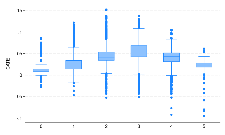
Note that catehat_S contains the CATE estimate from our S-learner. Figure 1(a) summarizes the results, where the potential voters are grouped by their voting history. It shows the distribution of CATE estimates for each of the subgroups. These results can help campaign organizers better target mailers in the future. For instance, if resources are limited, focusing on potential voters who voted three times during the past five elections may be most effective. This group not only exhibits the highest estimated ATE but also represents the largest segment of potential voters, making it an ideal target for maximizing impact.
|
|
|
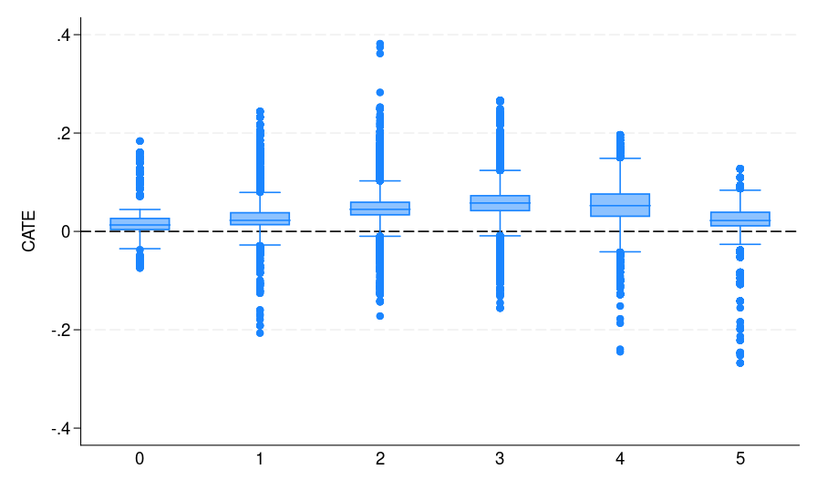
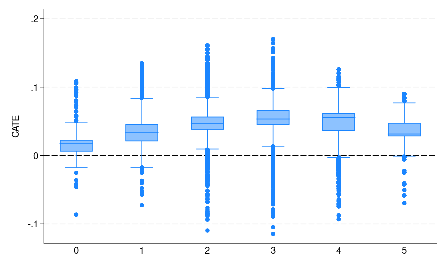
| (a) S-learner | (b) T-learner | (c) X-learner |
| Figure 1: The CATE estimate distribution for each bin, where potential voters are grouped by the number of elections they participated in | ||
Explainable machine learning for CATE
Machine learning models are often treated as black boxes that do not explain their predictions in a way that practitioners can understand. Explainable machine learning refers to methods that rely on external models to make the decisions and predictions of those models presentable and understandable to a human.
The discussion in this section applies to all types of learning methods discussed in this blog. For illustration, we show only the S-learner. Having CATE estimates from the previous sections, we can build a surrogate model, for example, GBM, for CATE using the predictors and use the available explainable method in the h2oml suite of commands to explain CATE predictions. For available, explainable commands, see Interpretation and explanation in [H2OML] Intro.
To demonstrate, we will focus on exploring SHAP values and creating a partial dependence plot. We start by uploading the current dataset in Stata as an H2O frame. Then, to make sure that the factor variables have a correct H2O type enum, we use the _h2oframe factor command with the replace option. Then, we run gradient boosting regression for the estimated CATEs in catehat_S. As mentioned above, we suggest tuning this model as well.
. _h2oframe put, into(social_cat) current
(output omitted)

. _h2oframe factor gender g2000 g2002 p2000 p2002 p2004 treatment, replace

. h2oml gbregress catehat_S $predictors, h2orseed(19)
(output omitted)
We graph the SHAP values and create a partial dependence plot (PDP) for explainability.
. h2omlgraph shapvalues, obs(5)

. h2omlgraph pdp age
(output omitted)
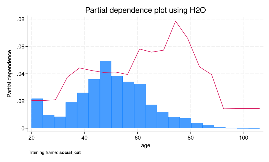
Figure 2 presents both SHAP values for an individual prediction and a PDP for age. For SHAP values, we explain the fifth observation, which corresponds to a female who is 39 years old. We can see that the age of 39 and voting in the 2002 general elections but not voting in the 2000 primary elections contribute positively to explaining the difference between the individual’s CATE prediction (0.0482) and the average prediction of 0.0437. However, not voting in the 2004 primary elections had a negative contribution.
From the PDP, the red line shows an increase in predicted CATE between ages 30 and 40, followed by a small decrease and then an increase from around age 60 to 80. One possible interpretation of the plateau and modest dip between 40 and 60 is that individuals in that age group may exhibit more stable voting patterns that are harder to influence using social pressure mailers.
We could similarly explore SHAP values for other individuals and PDP plots for other predictors.
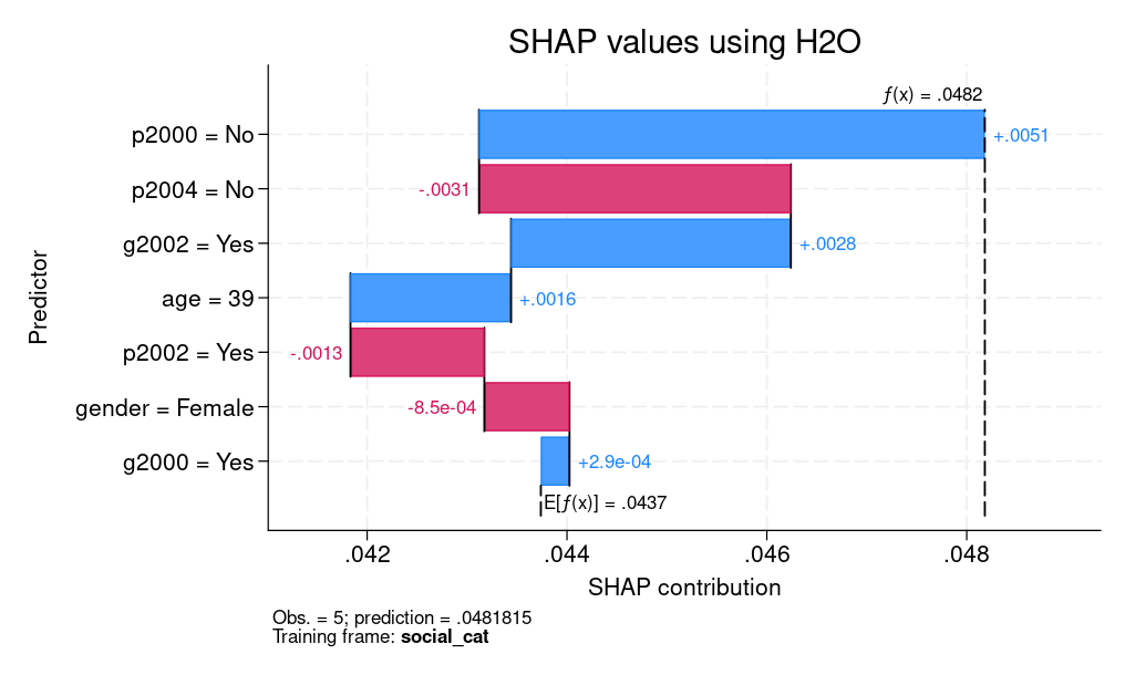
|
|
| (a) SHAP values | (b) PDP |
| Figure 2: Explainable machine learning for CATE: (a) SHAP values (b) PDP | |
Next we demonstrate how to implement the T-learner. We begin by splitting the dataset into two H2O frames: one for control observations (social0) and another for treated observations (social1). These frames will be used to fit separate models for predicting outcomes in the treated and control groups, as described in appendix A.2.
. // T-learner step 1: Split data by treatment group
. frame change social

. _h2oframe put if treatment == 0, into(social0) replace // control group
(output omitted)

. _h2oframe put if treatment == 1, into(social1) replace // treated group
(output omitted)
Next we use the h2oml gbbinclass command to train a gradient boosting binary classification model on the control group data, with voted as the outcome. The predictor names are specified using the predictors macro, defined earlier. We store this model using h2omlest store so we can later reload it for predictions in the next section.
. // T-learner step 2: Train a GBM model for the control response function
. _h2oframe change social0

. h2oml gbbinclass voted $predictors, h2orseed(19) // GBM model: predict voting for T=group (control)
(output omitted)

. h2omlest store M0                                // Store model as MO

. h2omlpredict yhat0_0 yhat0_1, frame(social) pr   // Predict yhat0_1 = Pr(Y=1|X,T=0) based on model MO for full sample

Progress (%): 0 100
After training the control model, we switch to the treated group frame and train another GBM model, again using voted as the outcome. This model is stored separately and represents our estimate of the treatment response function.
. // T-learner step 3: Train a GBM model for the treatment response function
. _h2oframe change social1

. h2oml gbbinclass voted $predictors, h2orseed(19) // GBM model: predict voting for T=1 group (treated)
(output omitted)

. h2omlest store M1                                // Store model as M1

. h2omlpredict yhat1_0 yhat1_1, frame(social) pr   // Predict yhat1_1 = Pr(Y=1|X,T=1) based on model M1 for full sample

Progress (%): 0 100
Once both models are trained, we use them to generate counterfactual predictions yhat0_1 and yhat1_1 for all individuals in the full dataset. These predictions correspond to \(\hat{\mu}_0(\mathbf{x})\) and \(\hat{\mu}_1(\mathbf{x})\) in \eqref{eq:catetlearner} in appendix A.2. We then compute their difference in Stata and store it as catehat_T, which corresponds to the T-learner estimate of CATE \(\hat{\tau}_T(\mathbf{x})\). Last, we plot the distribution of the CATE estimates by voting history [figure 1(b)] to assess how treatment effects vary across subgroups. It can be seen that both S- and T-learners (also the X-learner) provide similar CATE estimates.
. // T-learner step 4: Estimate CATE and visualize
. frame change default

. _h2oframe get yhat1_1 yhat0_1 totalvote using social, clear

. generate double catehat_T = yhat1_1 - yhat0_1  // CATE = treated prediction - control prediction

. graph box catehat_T, over(totalvote) yline(0) ytitle("CATE")
The X-learner begins by using the previously trained outcome models, M0 and M1 from the T-learner, to generate counterfactual predictions. Specifically, we use the control group model to predict what treated individuals would have done under control [\(\hat{\mu}_0(X_i^1)\)] and the treated group model to predict what control individuals would have done under treatment [\(\hat{\mu}_1(X_i^0)\)].
. // X-learner step 1: Predict counterfactual outcomes for treated units
. h2omlest restore M0                              // Restore (load) control model

. h2omlpredict yhat0_0 yhat0_1, frame(social1) pr  // Predict yhat0_1 = Pr(Y=1|X,T=0) for treated units

Progress (%): 0 100

. // X-learner step 2: Predict counterfactual outcomes for control units
. h2omlest restore M1                              // Restore (load) treated model
(results M1 are active now)

. h2omlpredict yhat1_0 yhat1_1, frame(social0) pr // Predict yhat1_1 = Pr(Y=1|X,T=1) for control units

Progress (%): 0 100
Next we compute imputed treatment effects by subtracting these counterfactual predictions from observed outcomes. For treated individuals, this is \(\tilde{D}_i^1 = Y^1_i – \hat{\mu}_0(X^1_i)\), and for control individuals, it is \(\tilde{D}_i^0 = \hat{\mu}_1(X^0_i) – Y^0_i\). These imputed effects serve as pseudooutcomes in the second stage of the X-learner. We then fit regression models using h2oml gbregress to predict these pseudooutcomes \(\tilde{D}_i^1\) and \(\tilde{D}_i^0\) using the original covariates. These correspond to \(\hat{\tau}_1(\mathbf{x})\) and \(\hat{\tau}_0(\mathbf{x})\) in \eqref{eq:catexlearner} in appendix A.3, which are the estimated CATE functions derived from the treated and control groups, respectively.
. // X-learner step 3: Impute treatment effects for treated units
. _h2oframe change social1

. _h2oframe tonumeric voted, replace           // Ensure `voted' is numeric

. _h2oframe generate D1 = voted - yhat0_1      // Imputed effect = Y - counterfactual

. h2oml gbregress D1 $predictors, h2orseed(19) // Model-imputed treatment effects
(output omitted)

. h2omlpredict cate1, frame(social)            // Predict cate1(x) = E(D1|X=x) on full sample

. // X-learner step 4: Impute treatment effects for control units
. _h2oframe change social0

. _h2oframe tonumeric voted, replace

. _h2oframe generate D0 = yhat1_1 - voted      // Imputed effect = counterfactual - Y

. h2oml gbregress D0 $predictors, h2orseed(19)
(output omitted)

. h2omlpredict cate0, frame(social)            // Predict cate0(x) = E(D0|X=x) on full sample
Finally, we combine these two CATE estimates stored in cate1 and cate0 using a weighted average. In line with Künzel et al. (2019), we use a fixed weight \(g(x)=0.5\) for simplicity, although in practice this can be set to the estimated propensity score \(\hat{e}(\mathbf{x})\).
. // X-learner step 5: Combine CATE estimates from both groups
. _h2oframe get cate0 cate1 totalvote using social, clear

. local gx = 0.5                                                // Combine with weight (0.5 here, could be e(x))

. generate double catehat_X = `gx' * cate0 + (1 - `gx') * cate1 // Final CATE estimate

. graph box catehat_X, over(totalvote) yline(0) ytitle("CATE")
The distribution of the CATE estimates by voting history is displayed in figure 1(c).
As can be seen from figure 1, all S-, T-, and X-learners provide similar CATE estimates. This result is expected given the very large sample size and small number of predictors. Thus, it is informative to discuss when to adopt which learner. Following Künzel et al. (2019), we suggest using the S-learner when the researcher suspects that the treatment effect is simple or zero. If the treatment effect is strongly heterogeneous and the response outcome distribution varies between treatment and control groups, then the T-learner might perform well. Using various simulation settings, Künzel et al. (2019) show that the X-learner effectively adapts to these different settings and performs well even when the treatment and control groups are imbalanced.
A metalearner is a high-level algorithm that decomposes the CATE estimation problem into several regression tasks solvable by machine learning models (base learners like random forest, GBM, etc.).
Let \( Y^0 \) and \( Y^1 \) denote the observed outcomes for the control and treatment groups, respectively. For instance, \( Y^1_i \) is the outcome of the \( i \)th unit in the treatment group. Covariates are denoted by \( \mathbf{X}^0 \) and \( \mathbf{X}^1 \), where \( \mathbf{X}^0 \) corresponds to the covariates of control units and \( \mathbf{X}^1 \) to those of treated units; \( \mathbf{X}^1_i \) refers to the covariate vector for the \( i \)th treated unit. The treatment assignment indicator is denoted by \( T \in \{0, 1\} \), with \( T = 1 \) indicating treatment and \( T = 0 \) indicating control.
Regression models are represented using the notation \( M_k(Y \sim \mathbf{X}) \), which denotes a generic learning algorithm, possibly distinct across models, that estimates the conditional expectation \( \mathbb{E}(Y \mid \mathbf{X} = \mathbf{x}) \) for given inputs. These models can be any machine learning estimator, including flexible black-box learners. The main estimand of interest is the CATE \eqref{eq:cate}. This is the quantity all metalearners are designed to estimate.
From \eqref{eq:cate}, the most straightforward thing to do is to just implement a machine learning model for the conditional expectation \(E(Y|\mathbf{X}, T)\). The S-learner, where the “S” stands for single, fits a single model, using both \( \mathbf{X} \) and \( T \) as covariates:
\[
\mu(\mathbf{x}, t) = \mathbb{E}(Y \mid \mathbf{X} = \mathbf{x}, T = t) \quad\text{ which is estimated using }\quad M\{Y \sim (\mathbf{X}, T)\}
\]
The CATE estimator is given by
\[
\hat{\tau}_S(\mathbf{x}) = \hat{\mu}(\mathbf{x},1) – \hat{\mu}(\mathbf{x}, 0) \tag{2}\label{eq:cateslearner}
\]
In practice, the treatment \(T\) is often one-dimensional, while \(\mathbf{X}\) can be high-dimensional. Looking at the CATE estimator in \eqref{eq:cateslearner}, notice that the only input to \(\hat{\mu}\) that changes between the two terms is \(T\). Consequently, if the machine learning model used for estimation largely ignores \(T\) and primarily focuses on \(\mathbf{X}\), the resulting CATE could incorrectly be zero. The T-learner, discussed next, attempts to address this issue.
The question we are trying to answer is, How do we make sure that the model \(\hat{\mu}\) does not ignore \(T\)? Well, we can achieve this by training two different models for the treatment and control response functions \(\mu_1(\mathbf{x})\) and \(\mu_0(\mathbf{x})\), respectively. The T-learner, where the “T” stands for two, fits two separate models for the treatment and control groups:
\begin{align}
\mu_1(\mathbf{x}) &= \mathbb{E}\{Y(1) \mid \mathbf{X} = \mathbf{x}, T = 1\}, \quad \text{estimated via }\quad M_1(Y^1 \sim \mathbf{X}^1)\\
\mu_0(\mathbf{x}) &= \mathbb{E}\{Y(0) \mid \mathbf{X} = \mathbf{x}, T = 0\}, \quad \text{estimated via }\quad M_2(Y^0 \sim \mathbf{X}^0)
\end{align}
Then the CATE estimator is given by
\[
\hat{\tau}_T(\mathbf{x}) = \hat{\mu}_1(\mathbf{x}) – \hat{\mu}_0(\mathbf{x}) \tag{3}\label{eq:catetlearner}
\]
To ensure \(T\) isn’t overlooked, we train two separate statistical models. First, we divide our data: \((Y^1,\mathbf{X}^1)\) consists of observations where \(T= 1\), and \((Y^0,\mathbf{X}^0)\) of observations where \(T= 0\). Then, we train \(M_1(Y^1 \sim \mathbf{X}^1)\) to predict \(Y\) for the \(T=1\) group and \(M_2(Y^0 \sim \mathbf{X}^0)\) to predict \(Y\) for the group \(T= 0\).
While the T-learner helps overcome the limitations of the S-learner, it introduces a new drawback: it doesn’t utilize all available data when estimating \(M_1\) and \(M_2\). The X-learner, which we introduce next, addresses this by ensuring the entire dataset is used efficiently for CATE estimation.
We first present the steps, then demystify their motivation. The X-learner proceeds in four steps:
- Fit the outcome models:
\[
\hat{\mu}_0(x) \text{ using } M_1(Y^0 \sim \mathbf{X}^0) \; \text{and }\hat{\mu}_1(x) \text{ using } M_2(Y^1 \sim \mathbf{X}^1)
\] - Compute imputed treatment effects:
\[
\tilde{D}_i^1 = Y^1_i – \hat{\mu}_0(X^1_i), \quad \tilde{D}_i^0 = \hat{\mu}_1(X^0_i) – Y^0_i
\] - Fit the models to estimate:
\begin{align}
\tau_1(\mathbf{x}) &= \mathbb{E}(\tilde{D}^1 \mid \mathbf{X} = \mathbf{x}), \quad \text{estimated via } \quad M_3(\tilde{D}^1 \sim \mathbf{X}^1)\\
\tau_0(\mathbf{x}) &= \mathbb{E}(\tilde{D}^0 \mid \mathbf{X} = \mathbf{x}), \quad \text{estimated via } \quad M_4(\tilde{D}^0 \sim \mathbf{X}^0)
\end{align} - Combine estimates \(\hat{\tau}_0(\mathbf{x}) \) and \(\hat{\tau}_1(\mathbf{x}) \) to obtain the desired CATE estimator:
\[
\hat{\tau}_X(\mathbf{x}) = g(\mathbf{x}) \hat{\tau}_0(\mathbf{x}) + \{1 – g(\mathbf{x})\} \hat{\tau}_1(\mathbf{x}) \tag{4}\label{eq:catexlearner}
\]
where \( g(\mathbf{x}) \in [0,1] \) is a weight function whose goal is to minimize the variance of \(\tau(\mathbf{x})\). An estimator of the propensity score \( e(\mathbf{x}) = \mathbb{P}(T=1 \mid \mathbf{X}=\mathbf{x}) \) is one possible choice for \(g(\mathbf{x})\).
As can be seen, the first step of the X-learner is exactly the same as the T-learner. Separate regression models are fit to the treatment and control group data. The next two steps form the ingenuity of the method, because this is where all data from both models are utilized and where the “X” (cross-estimation) in X-learner derives its meaning. In step 2, \(\tilde{D}_i^1\) and \(\tilde{D}_i^0\) are the ITE estimates for the treatment and control groups, respectively. \(\tilde{D}_i^1\) uses the treatment group outcomes and the imputed counterfactual obtained from \(\hat{\mu}_0\) in step 1. Analogously, \(\tilde{D}_i^0\) is computed using the control group outcomes and the imputed counterfactual estimated from \(\hat{\mu}_1\). This latter step ensures that the ITE estimates for each group utilize data from both the treatment and control groups. However, each of the estimates \(\tilde{D}_i^1\) and \(\tilde{D}_i^0\) uses only a single observation from its corresponding group. To address this, the X-learner fits two different regression models in step 3, resulting in two estimates: \(\hat{\tau}_1(\mathbf{x})\), which intends to effectively estimate \(E(Y^1|\mathbf{X} = \mathbf{x})\), and \(\hat{\tau}_0(\mathbf{x})\), which intends to estimate \(E(Y^0|\mathbf{X} = \mathbf{x})\). Finally, step 4 combines these two estimates into a single CATE estimate. Depending on the dataset, the choice of the weight function \(g(\mathbf{x})\) may vary. If the sizes of the treatment and control groups differ significantly, one might choose \(g(\mathbf{x})=0\) or \(g(\mathbf{x})=1\) to prioritize one group’s estimate. In our analysis, we use \(g(x) = 0.5\) to equally weight the estimates from both groups.
References
Athey, S., J. Tibshirani, and S. Wager. 2019. Generalized random forests. Annals of Statistics 47: 1148–1178. https://doi.org/10.1214/18-AOS1709.
Gerber, A., D. P. Green, and C. W. Larimer. 2008. Social pressure and voter turnout: Evidence from a large-scale field experiment. American Political Science Review 102: 33–48. https://doi.org/10.1017/S000305540808009X.
Jacob, D. 2021. CATE meets ML: Conditional average treatment effect and machine learning. Discussion Papers 2021-005, Humboldt-Universität of Berlin, International Research Training Group 1792. High-Dimensional Nonstationary Time Series.
Künzel, S. R., J. S. Sekhon, P. J. Bickel, and B. Yu. 2019. Metalearners for estimating heterogeneous treatment effects using machine learning. Proceedings of the National Academy of Sciences 116: 4156–4165. https://doi.org/10.1073/pnas.1804597116.
Nie, X., and S. Wager. 2020. Quasi-oracle estimation of heterogeneous treatment effects. Biometrika 108: 299–319. https://doi.org/10.1093/biomet/asaa076.
Robins, J., L. Li, E. Tchetgen, and A. van der Vaart. 2008. Higher order influence functions and minimax estimation of nonlinear functionals. Institute of Mathematical Statistics Collections 2: 335–421. https://doi.org/10.1214/193940307000000527.
Robins, J. M., S. D. Mark, and W. K. Newey. 1992. Estimating exposure effects by the expectation of exposure conditional on confounders. Biometrics 48: 479–495.
Robins, J. M., and A. Rotnitzky. 1995. Semiparametric efficiency in multivariate regression models with missing data. Journal of the American Statistical Association 90 122–129. https://doi.org/10.2307/2291135.
van der Laan, M. J. 2006. Statistical inference for variable importance. International Journal of Biostatistics Art. 2. https://doi.org/10.2202/1557-4679.1008.
Vegetabile, B. G. 2021. On the distinction between “conditional average treatment effects” (CATE) and “individual treatment effects” (ITE) under ignorability assumptions. arXiv:2108.04939 [stat.ME]. https://doi.org/10.48550/arXiv.2108.04939.