Using resampling methods to detect influential points
As stated in the documentation for jackknife, an often forgotten utility for this command is the detection of overly influential observations.
Some commands, like logit or stcox, come with their own set of prediction tools to detect influential points. However, these kinds of predictions can be computed for virtually any regression command. In particular, we will see that the dfbeta statistics can be easily computed for any command that accepts the jackknife prefix. dfbeta statistics allow us to visualize how influential some observations are compared with the rest, concerning a specific parameter.
We will also compute Cook’s likelihood displacement, which is an overall measure of influence, and it can also be compared with a specific threshold.
Using jackknife to compute dfbeta
The main task of jackknife is to fit the model while suppressing one observation at a time, which allows us to see how much results change when each observation is suppressed; in other words, it allows us to see how much each observation influences the results. A very intuitive measure of influence is dfbeta, which is the amount that a particular parameter changes when an observation is suppressed. There will be one dfbeta variable for each parameter. If \(\hat\beta\) is the estimate for parameter \(\beta\) obtained from the full data and \( \hat\beta_{(i)} \) is the corresponding estimate obtained when the \(i\)th observation is suppressed, then the \(i\)th element of variable dfbeta is obtained as
\[dfbeta = \hat\beta – \hat\beta_{(i)}\]
Parameters \(\hat\beta\) are saved by the estimation commands in matrix e(b) and also can be obtained using the _b notation, as we will show below. The leave-one-out values \(\hat\beta_{(i)}\) can be saved in a new file by using the option saving() with jackknife. With these two elements, we can compute the dfbeta values for each variable.
Let’s see an example with the probit command.
. sysuse auto, clear
(1978 Automobile Data)
. *preserve original dataset
. preserve
. *generate a variable with the original observation number
. gen obs =_n
. probit foreign mpg weight
Iteration 0: log likelihood = -45.03321
Iteration 1: log likelihood = -27.914626
Iteration 2: log likelihood = -26.858074
Iteration 3: log likelihood = -26.844197
Iteration 4: log likelihood = -26.844189
Iteration 5: log likelihood = -26.844189
Probit regression Number of obs = 74
LR chi2(2) = 36.38
Prob > chi2 = 0.0000
Log likelihood = -26.844189 Pseudo R2 = 0.4039
------------------------------------------------------------------------------
foreign | Coef. Std. Err. z P>|z| [95% Conf. Interval]
-------------+----------------------------------------------------------------
mpg | -.1039503 .0515689 -2.02 0.044 -.2050235 -.0028772
weight | -.0023355 .0005661 -4.13 0.000 -.003445 -.0012261
_cons | 8.275464 2.554142 3.24 0.001 3.269437 13.28149
------------------------------------------------------------------------------
. *keep the estimation sample so each observation will be matched
. *with the corresponding replication
. keep if e(sample)
(0 observations deleted)
. *use jackknife to generate the replications, and save the values in
. *file b_replic
. jackknife, saving(b_replic, replace): probit foreign mpg weight
(running probit on estimation sample)
Jackknife replications (74)
----+--- 1 ---+--- 2 ---+--- 3 ---+--- 4 ---+--- 5
.................................................. 50
........................
Probit regression Number of obs = 74
Replications = 74
F( 2, 73) = 10.36
Prob > F = 0.0001
Log likelihood = -26.844189 Pseudo R2 = 0.4039
------------------------------------------------------------------------------
| Jackknife
foreign | Coef. Std. Err. t P>|t| [95% Conf. Interval]
-------------+----------------------------------------------------------------
mpg | -.1039503 .0831194 -1.25 0.215 -.269607 .0617063
weight | -.0023355 .0006619 -3.53 0.001 -.0036547 -.0010164
_cons | 8.275464 3.506085 2.36 0.021 1.287847 15.26308
------------------------------------------------------------------------------
. *verify that all the replications were successful
. assert e(N_misreps) ==0
. merge 1:1 _n using b_replic
Result # of obs.
-----------------------------------------
not matched 0
matched 74 (_merge==3)
-----------------------------------------
. *see how values from replications are stored
. describe, fullnames
Contains data from .../auto.dta
obs: 74 1978 Automobile Data
vars: 17 13 Apr 2013 17:45
size: 4,440 (_dta has notes)
--------------------------------------------------------------------------------
storage display value
variable name type format label variable label
--------------------------------------------------------------------------------
make str18 %-18s Make and Model
price int %8.0gc Price
mpg int %8.0g Mileage (mpg)
rep78 int %8.0g Repair Record 1978
headroom float %6.1f Headroom (in.)
trunk int %8.0g Trunk space (cu. ft.)
weight int %8.0gc Weight (lbs.)
length int %8.0g Length (in.)
turn int %8.0g Turn Circle (ft.)
displacement int %8.0g Displacement (cu. in.)
gear_ratio float %6.2f Gear Ratio
foreign byte %8.0g origin Car type
obs float %9.0g
foreign_b_mpg float %9.0g [foreign]_b[mpg]
foreign_b_weight
float %9.0g [foreign]_b[weight]
foreign_b_cons float %9.0g [foreign]_b[_cons]
_merge byte %23.0g _merge
--------------------------------------------------------------------------------
Sorted by:
Note: dataset has changed since last saved
. *compute the dfbeta for each covariate
. foreach var in mpg weight {
2. gen dfbeta_`var' = (_b[`var'] -foreign_b_`var')
3. }
. gen dfbeta_cons = (_b[_cons] - foreign_b_cons)
. label var obs "observation number"
. label var dfbeta_mpg "dfbeta for mpg"
. label var dfbeta_weight "dfbeta for weight"
. label var dfbeta_cons "dfbeta for the constant"
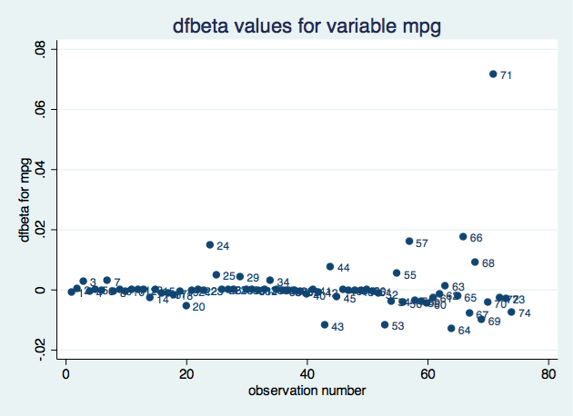
. *plot dfbeta values for variable mpg
. scatter dfbeta_mpg obs, mlabel(obs) title("dfbeta values for variable mpg")
. *restore original dataset
. restore

Based on the impact on the coefficient for variable mpg, observation 71 seems to be the most influential. We could create a similar plot for each parameter.
jackknife prints a dot for each successful replication and an ‘x’ for each replication that ends with an error. By looking at the output immediately following the jackknife command, we can see that all the replications were successful. However, we added an assert line in the code to avoid relying on visual inspection. If some replications failed, we would need to explore the reasons.
A computational shortcut to obtain the dfbeta values
The command jackknife allows us to save the leave-one-out values in a different file. To use these, we would need to do some data management and merge the two files. On the other hand, the same command called with the option keep saves pseudovalues, which are defined as follows:
\[\hat{\beta}_i^* = N\hat\beta – (N-1)\hat\beta_{(i)} \]
where \(N\) is the number of observations involved in the computation, returned as e(N). Therefore, using the pseudovalues, \(\beta_{(i)}\) values can be computed as \[\hat\beta_{(i)} = \frac{ N \hat\beta – \hat\beta^*_i}{N-1} \]
Also, dfbeta values can be computed directly from the pseudovalues as \[ \hat\beta – \hat\beta_{(i)} = \frac{\hat\beta_{i}^* -\hat\beta} {N-1} \]
Using the pseudovalues instead of the leave-one-out values simplifies our program because we don’t have to worry about matching each pseudovalue to the correct observation.
Let’s reproduce the previous example.
. sysuse auto, clear
(1978 Automobile Data)

. jackknife, keep: probit foreign  mpg weight
(running probit on estimation sample)

Jackknife replications (74)
----+--- 1 ---+--- 2 ---+--- 3 ---+--- 4 ---+--- 5
..................................................    50
........................

Probit regression                               Number of obs      =        74
                                                Replications       =        74
                                                F(   2,     73)    =     10.36
                                                Prob > F           =    0.0001
Log likelihood = -26.844189                     Pseudo R2          =    0.4039

------------------------------------------------------------------------------
             |              Jackknife
     foreign |      Coef.   Std. Err.      t    P>|t|     [95% Conf. Interval]
-------------+----------------------------------------------------------------
         mpg |  -.1039503   .0831194    -1.25   0.215     -.269607    .0617063
      weight |  -.0023355   .0006619    -3.53   0.001    -.0036547   -.0010164
       _cons |   8.275464   3.506085     2.36   0.021     1.287847    15.26308
------------------------------------------------------------------------------

. *see how pseudovalues are stored
. describe, fullnames

Contains data from /Users/isabelcanette/Desktop/stata_mar18/309/ado/base/a/auto.
> dta
  obs:            74                          1978 Automobile Data
 vars:            15                          13 Apr 2013 17:45
 size:         4,070                          (_dta has notes)
--------------------------------------------------------------------------------
              storage   display    value
variable name   type    format     label      variable label
--------------------------------------------------------------------------------
make            str18   %-18s                 Make and Model
price           int     %8.0gc                Price
mpg             int     %8.0g                 Mileage (mpg)
rep78           int     %8.0g                 Repair Record 1978
headroom        float   %6.1f                 Headroom (in.)
trunk           int     %8.0g                 Trunk space (cu. ft.)
weight          int     %8.0gc                Weight (lbs.)
length          int     %8.0g                 Length (in.)
turn            int     %8.0g                 Turn Circle (ft.)
displacement    int     %8.0g                 Displacement (cu. in.)
gear_ratio      float   %6.2f                 Gear Ratio
foreign         byte    %8.0g      origin     Car type
foreign_b_mpg   float   %9.0g                 pseudovalues: [foreign]_b[mpg]
foreign_b_weight
                float   %9.0g                 pseudovalues: [foreign]_b[weight]
foreign_b_cons  float   %9.0g                 pseudovalues: [foreign]_b[_cons]
--------------------------------------------------------------------------------
Sorted by:  foreign
     Note:  dataset has changed since last saved

. *verify that all the replications were successful
. assert e(N_misreps)==0

. *compute the dfbeta for each covariate
. local N = e(N)

. foreach var in  mpg weight {
  2. gen dfbeta_`var' = (foreign_b_`var' - _b[`var'])/(`N'-1)
  3. }

. gen dfbeta_`cons' = (foreign_b_cons - _b[_cons])/(`N'-1)

. *plot deff values for variable weight
. gen obs = _n

. label var obs "observation number"

. label var dfbeta_mpg "dfbeta for mpg"

. scatter dfbeta_mpg obs, mlabel(obs) title("dfbeta values for variable mpg")
Dfbeta for grouped data
If you have panel data or a situation where each individual is represented by a group of observations (for example, conditional logit or survival models), you might be interested in influential groups. In this case, you would look at the changes on the parameters when each group is suppressed. Let’s see an example with xtlogit.
. webuse towerlondon, clear
. xtset family

. jackknife, cluster(family) idcluster(newclus) keep: xtlogit dtlm difficulty
. assert e(N_misreps)==0
The group-level pseudovalues will be saved on the first observations corresponding to each group, and there will be missing values on the rest. To compute the dfbeta value for the coefficient for difficulty, we type
. local N = e(N_clust)
. gen dfbeta_difficulty = (dtlm_b_difficulty - _b[difficulty])/(`N'-1)
We can then plot those values:
. scatter dfbeta_difficulty newclus, mlabel(family) ///
       title("dfbeta values for variable difficulty") xtitle("family")
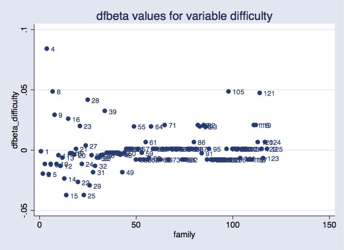
Option idcluster() for jackknife generates a new variable that assigns consecutive integers to the clusters; using this variable produces a plot where families are equally spaced on the horizontal axis.
As before, we can see that some groups are more influential than others. It would require some research to find out whether this is a problem.
Likelihood displacement
If we want a global measure of influence (that is, not tied to a particular parameter), we can compute the likelihood displacement values. We consider the likelihood displacement value as defined by Cook (1986):
\[LD_i = 2[L(\hat\theta) – L(\hat\theta_{(i)})] \]
where \(L\) is the log-likelihood function (evaluated on the full dataset), \(\hat\theta\) is the set of parameter estimates obtained from the full dataset, and \(\hat\theta_{(i)}\) is the set of the parameter estimates obtained when leaving out the \(i\)th observation. Notice that what changes is the parameter vector. The log-likelihood function is always evaluated on the whole sample; provided that \(\hat\theta\) is the set of parameters that maximizes the log likelihood, the log-likelihood displacement is always positive. Cook suggested, as a confidence region for this value, the interval \([0, \chi^2_p(\alpha))\), where \(\chi^2_p(\alpha)\) is the (\(1-\alpha\)) quantile from a chi-squared distribution with \(p\) degrees of freedom, and \(p\) is the number of parameters in \(\theta\).
To perform our assessment based on the likelihood displacement, we will need to do the following:
- Create an \(N\times p\) matrix B, where the \(i\)th row contains the vector of parameter estimates obtained by leaving the \(i\)th observation out.
- Create a new variable L1 such that its \(i\)th observation contains the log likelihood evaluated at the parameter estimates in the \(i\)th row of matrix B.
- Use variable L1 to obtain the LD matrix, containing the likelihood displacement values.
- Construct a plot for the values in LD, and add the \(\chi^2_p(\alpha)\) as a reference.
Let’s do it with our probit model.
Step 1.
We first create the macro cmdline containing the command line for the model we want to use. We fit the model and save the original log likelihood in macro ll0.
With a loop, the leave-one-out parameters are saved in consecutive rows of matrix B. It is useful to have those values in a matrix, because we will then extract each row to evaluate the log likelihood at those values.
**********Step 1
sysuse auto, clear
set more off
local cmdline probit foreign weight mpg
`cmdline'
keep if e(sample)
local ll0 = e(ll)
mat b0 = e(b)
mat b = b0

local N = _N

forvalues i = 1(1)`N'{
   `cmdline' if _n !=`i'
   mat b1 = e(b)
   mat b = b \ b1
}

mat B = b[2...,1...]
mat list B
Step 2.
In each iteration of a loop, a row from B is stored as matrix b. To evaluate the log likelihood at these values, the trick is to use them as initial values and invoke the command with 0 iterations. This can be done for any command that is based on ml.
**********Step 2

gen L1 = .

forvalues i = 1(1)`N'{
    mat b = B[`i',1...]
    `cmdline', from(b) iter(0)
    local ll = e(ll)
    replace L1 = `ll' in `i'
}
Step 3.
Using variable L1 and the macro with the original log likelihood, we compute Cook’s likehood displacement.
**********Step 3

gen LD = 2*(`ll0' - L1)
Step 4.
Create the plot, using as a reference the 90% quantile for the \(\chi^2\) distribution. \(p\) is the number of columns in matrix b0 (or equivalently, the number of columns in matrix B).
**********Step 4

local k = colsof(b0)
gen upper_bound = invchi2tail(`k', .1)
gen n = _n

twoway scatter LD n, mlabel(n) || line upper_bound n, ///
title("Likelihood displacement")
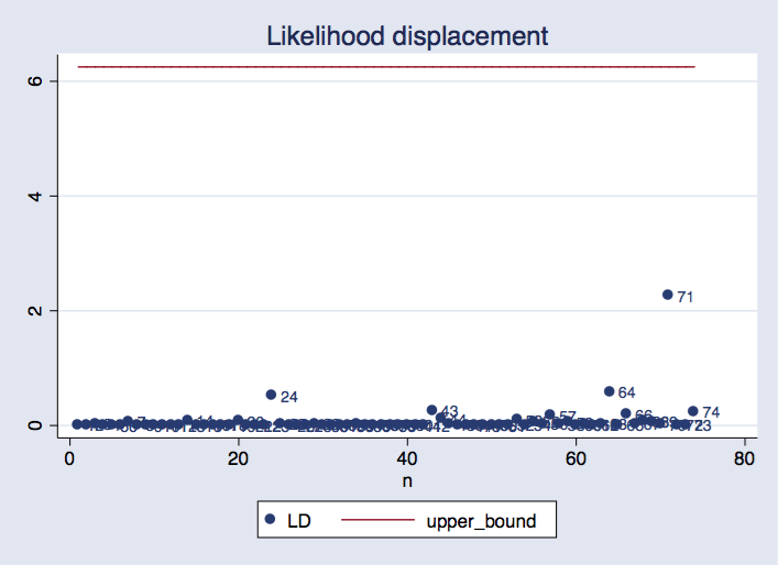
We can see that observation 71 is the most influential, and its likelihood displacement value is within the range we would normally expect.
Reference
Cook, D. 1986. Assessment of local influence. Journal of the Royal Statistical Society, Series B 48: 133–169.