Vector autoregression—simulation, estimation, and inference in Stata
\(\newcommand{\epsb}{{\boldsymbol{\epsilon}}}
\newcommand{\mub}{{\boldsymbol{\mu}}}
\newcommand{\thetab}{{\boldsymbol{\theta}}}
\newcommand{\Thetab}{{\boldsymbol{\Theta}}}
\newcommand{\etab}{{\boldsymbol{\eta}}}
\newcommand{\Sigmab}{{\boldsymbol{\Sigma}}}
\newcommand{\Phib}{{\boldsymbol{\Phi}}}
\newcommand{\Phat}{\hat{{\bf P}}}\)Vector autoregression (VAR) is a useful tool for analyzing the dynamics of multiple time series. VAR expresses a vector of observed variables as a function of its own lags.
Simulation
Let’s begin by simulating a bivariate VAR(2) process using the following specification,
\[
\begin{bmatrix} y_{1,t}\\ y_{2,t}
\end{bmatrix}
= \mub + {\bf A}_1 \begin{bmatrix} y_{1,t-1}\\ y_{2,t-1}
\end{bmatrix} + {\bf A}_2 \begin{bmatrix} y_{1,t-2}\\ y_{2,t-2}
\end{bmatrix} + \epsb_t
\]
where \(y_{1,t}\) and \(y_{2,t}\) are the observed series at time \(t\), \(\mub\) is a \(2 \times 1\) vector of intercepts, \({\bf A}_1\) and \({\bf A}_2\) are \(2\times 2\) parameter matrices, and \(\epsb_t\) is a \(2\times 1\) vector of innovations that is uncorrelated over time. I assume a \(N({\bf 0},\Sigmab)\) distribution for the innovations \(\epsb_t\), where \(\Sigmab\) is a \(2\times 2\) covariance matrix.
I set my sample size to 1,100 and generate variables to hold the observed series and innovations.
. clear all

. set seed 2016

. local T = 1100

. set obs `T'
number of observations (_N) was 0, now 1,100

. gen time = _n

. tsset time
        time variable:  time, 1 to 1100
                delta:  1 unit

. generate y1 = .
(1,100 missing values generated)

. generate y2 = .
(1,100 missing values generated)

. generate eps1 = .
(1,100 missing values generated)

. generate eps2 = .
(1,100 missing values generated)
In lines 1–6, I set the seed for the random-number generator, set my sample size to 1,100, and generate a time variable, time. In the remaining lines, I generate variables y1, y2, eps1, and eps2 to hold the observed series and innovations.
Setting parameter values
I choose the parameter values for the VAR(2) model as follows:
\[
\mub = \begin{bmatrix} 0.1 \\ 0.4 \end{bmatrix}, \quad {\bf A}_1 =
\begin{bmatrix} 0.6 & -0.3 \\ 0.4 & 0.2 \end{bmatrix}, \quad {\bf A}_2 =
\begin{bmatrix} 0.2 & 0.3 \\ -0.1 & 0.1 \end{bmatrix}, \quad \Sigmab =
\begin{bmatrix} 1 & 0.5 \\ 0.5 & 1 \end{bmatrix}
\]
. mata:
------------------------------------------------- mata (type end to exit) -----
: mu = (0.1\0.4)

: A1 = (0.6,-0.3\0.4,0.2)

: A2 = (0.2,0.3\-0.1,0.1)

: Sigma = (1,0.5\0.5,1)

: end
-------------------------------------------------------------------------------
In Mata, I create matrices mu, A1, A2, and Sigma to hold the parameter values. Before generating my data, I check whether these values correspond to a stable VAR(2) process. Let
\[
{\bf F} = \begin{bmatrix} {\bf A}_1 & {\bf A_2} \\ {\bf I}_2 & {\bf 0}
\end{bmatrix}
\]
denote a \(4\times 4\) matrix where \({\bf I}_2\) is a \(2\times 2\) identity matrix and \({\bf 0}\) is a \(2\times 2\) matrix of zeros. The VAR(2) process is stable if the modulus of all eigenvalues of \({\bf F}\) is less than 1. The code below computes the eigenvalues.
. mata:
------------------------------------------------- mata (type end to exit) -----
: K = p = 2               // K = number of variables; p = number of lags

: F = J(K*p,K*p,0)

: F[1..2,1..2] = A1

: F[1..2,3..4] = A2

: F[3..4,1..2] = I(K)

: X = L = .

: eigensystem(F,X,L)

: L'
                              1
    +----------------------------+
  1 |                .858715598  |
  2 |  -.217760515 + .32727213i  |
  3 |  -.217760515 - .32727213i  |
  4 |                .376805431  |
    +----------------------------+

: end
-------------------------------------------------------------------------------
I construct the matrix F as defined above and use the function eigensystem() to compute its eigenvalues. The matrix X holds the eigenvectors, and L holds the eigenvalues. All eigenvalues in L are less than 1. The modulus of the second and third complex eigenvalues is \(\sqrt{r^2 + c^2} = 0.3931\), where \(r\) is the real part and \(c\) is the complex part. After checking the stability condition, I generate draws for the VAR(2) model.
Drawing innovations from a multivariate normal
I draw random normal values from \(N({\bf 0},\Sigmab)\) and assign them to Stata variables eps1 and eps2.
. mata:
------------------------------------------------- mata (type end to exit) -----
: T = strtoreal(st_local("T"))

: u = rnormal(T,2,0,1)*cholesky(Sigma)

: epsmat = .

: st_view(epsmat,.,"eps1 eps2")

: epsmat[1..T,.] = u

: end
-------------------------------------------------------------------------------
I assign the sample size, defined in Stata as a local macro T, to a Mata numeric variable. This simplifies changing the sample size in the future; I only need to do this once at the beginning. In Mata, I use two functions: st_local() and strtoreal() to assign the sample size. The first function obtains strings from Stata macros, and the second function converts them into a real value.
The second line draws a \(1100 \times 2\) matrix of normal errors from a \(N({\bf 0},\Sigmab)\) distribution. I use the st_view() function to assign the draws to the Stata variables eps1 and eps2. This function creates a matrix that is a view on the current Stata dataset. I create a null matrix epsmat and use st_view() to modify epsmat based on the values of the Stata variables eps1 and eps2. Finally, I assign this matrix to hold the draws stored in u, effectively populating the Stata variables eps1 and eps2 with the random draws.
Generating the observed series
Following Lütkepohl (2005, 708), I generate the first two observations so that their correlation structure is the same as the rest of the sample. I assume a bivariate normal distribution with mean equal to the unconditional mean \(\thetab = ({\bf I}_K – {\bf A}_1 – {\bf A}_2)^{-1}\mub\). The covariance matrix of the first two observations of the two series is
\[
\text{vec}(\Sigmab_y) = ({\bf I}_{16} – {\bf F} \otimes {\bf F})^{-1}\text{vec}(\Sigmab_{\epsilon})
\]
where \(\text{vec}()\) is an operator that stacks matrix columns, \({\bf I}_{16}\) is a \(16\times 16\) identity matrix, and \(\Sigmab_{\epsilon} = \begin{bmatrix} \Sigmab & {\bf 0}\\ {\bf 0} & {\bf 0} \end{bmatrix}\) is a \(4\times 4\) matrix. The first two observations are generated as
\[
\begin{bmatrix} {\bf y}_0 \\ {\bf y}_{-1} \end{bmatrix} = {\bf Q} \etab + \Thetab
\]
where Q is a \(4\times 4\) matrix such that \({\bf QQ}’ = \Sigmab_y\), \(\etab\) is a \(4\times 1\) vector of standard normal innovations and \(\Thetab = \begin{bmatrix} \thetab \\ \thetab \end{bmatrix}\) is a \(4\times 1\) vector of means.
The following code generates the first two observations and assigns the values to the Stata variables y1 and y2.
. mata:
------------------------------------------------- mata (type end to exit) -----
: Sigma_e = J(K*p,K*p,0)

: Sigma_e[1..K,1..K] = Sigma

: Sigma_y = luinv(I((K*p)^2)-F#F)*vec(Sigma_e)

: Sigma_y = rowshape(Sigma_y,K*p)'

: theta = luinv(I(K)-A1-A2)*mu

: Q = cholesky(Sigma_y)*rnormal(K*p,1,0,1)

: data = .

: st_view(data,.,"y1 y2")

: data[1..p,.] = ((Q[3..4],Q[1..2]):+mu)'

: end
-------------------------------------------------------------------------------
After generating the first two observations, I can generate the rest of the series from a VAR(2) process in Stata as follows:
. forvalues i=3/`T' {
  2.         qui {
  3. replace y1 = 0.1 + 0.6*l.y1 - 0.3*l.y2 + 0.2*l2.y1 + 0.3*l2.y2 + eps1 in `
> i'
  4. replace y2 = 0.4 + 0.4*l.y1 + 0.2*l.y2 - 0.1*l2.y1 + 0.1*l2.y2 + eps2 in `
> i'
  5.         }
  6. }

. drop in 1/100
(100 observations deleted)
I added the quietly statement to suppress the output generated after the replace command. Finally, I drop the first 100 observations as burn-in to mitigate the effect of initial values.
Estimation
I use the var command to fit a VAR(2) model.
. var y1 y2

Vector autoregression

Sample:  103 - 1100                             Number of obs     =        998
Log likelihood =  -2693.949                     AIC               =   5.418735
FPE            =   .7733536                     HQIC              =    5.43742
Det(Sigma_ml)  =   .7580097                     SBIC              =   5.467891

Equation           Parms      RMSE     R-sq      chi2     P>chi2
----------------------------------------------------------------
y1                    5     1.14546   0.5261   1108.039   0.0000
y2                    5     .865602   0.4794   919.1433   0.0000
----------------------------------------------------------------

------------------------------------------------------------------------------
             |      Coef.   Std. Err.      z    P>|z|     [95% Conf. Interval]
-------------+----------------------------------------------------------------
y1           |
          y1 |
         L1. |   .5510793   .0324494    16.98   0.000     .4874797     .614679
         L2. |   .2749983   .0367192     7.49   0.000       .20303    .3469667
             |
          y2 |
         L1. |  -.3080881    .046611    -6.61   0.000    -.3994439   -.2167323
         L2. |   .2551285   .0425803     5.99   0.000     .1716727    .3385844
             |
       _cons |   .1285357   .0496933     2.59   0.010     .0311387    .2259327
-------------+----------------------------------------------------------------
y2           |
          y1 |
         L1. |   .3890191   .0245214    15.86   0.000      .340958    .4370801
         L2. |  -.0190324    .027748    -0.69   0.493    -.0734175    .0353527
             |
          y2 |
         L1. |   .1944531    .035223     5.52   0.000     .1254172     .263489
         L2. |   .0459445   .0321771     1.43   0.153    -.0171215    .1090106
             |
       _cons |   .4603854   .0375523    12.26   0.000     .3867843    .5339865
------------------------------------------------------------------------------
By default, var estimates the parameters of a VAR model with two lags. The parameter estimates are significant and are similar to the true values used to generate the bivariate series.
Inference: Impulse response functions
Impulse response functions (IRF) are useful to analyze the response of endogenous variables in the VAR model due to an exogenous impulse to one of the innovations. For example, in a bivariate VAR of inflation and interest rate, IRFs can trace out the response of interest rates over time due to exogenous shocks to the inflation equation.
Let’s consider the bivariate model that I used earlier. Suppose I want to estimate the effect of a unit shock in \(\epsb_t\) to the endogenous variables in my system. I do this by converting the VAR(2) process into an MA(\(\infty\)) process
as
\[
{\bf y}_t = \sum_{p=0}^\infty \Phib_p \mub + \sum_{p=0}^\infty \Phib_p \epsb_{t-p}
\]
where \(\Phib_p\) is the MA(\(\infty\)) coefficient matrices for the pth lag. Following Lütkepohl (2005, 22–23), the MA coefficient matrices are related to the AR matrices as follows:
\begin{align*}
\Phib_0 &= {\bf I}_2 \\
\Phib_1 &= {\bf A}_1 \\
\Phib_2 &= \Phib_1 {\bf A}_1 + {\bf A}_2 = {\bf A}_1^2 + {\bf A}_2\\
&\vdots \\
\Phib_i &= \Phib_{i-1} {\bf A}_1 + \Phib_{i-2}{\bf A}_2
\end{align*}
More formally, the future \(h\) responses of the ith variable due to a unit shock in the jth equation at time \(t\) are given by
\[
\frac{\partial y_{i,t+h}}{\partial \epsilon_{j,t}} = \{\Phib_h\}_{i,j}
\]
The responses are the collection of elements in the ith row and jth column of the MA(\(\infty\)) coefficient matrices. For the VAR(2) model, the first few responses using the estimated AR parameters are as follows:
\begin{align*}
\begin{bmatrix} y_{1,0} \\ y_{2,0} \end{bmatrix} &=
\Phib_0 = {\bf I}_2 =
\begin{bmatrix} 1 & 0\\ 0 & 1 \end{bmatrix} \\
\begin{bmatrix} y_{1,1} \\ y_{2,1} \end{bmatrix} &=
\hat{\Phib}_1 = \hat{{\bf A}}_1 =
\begin{bmatrix} 0.5510 & -0.3081 \\ 0.3890 & 0.1945 \end{bmatrix} \\
\begin{bmatrix} y_{1,2} \\ y_{2,2} \end{bmatrix} &= \hat{\Phib}_2 =
\hat{{\bf A}}_1^2 + \hat{{\bf A}}_2 =
\begin{bmatrix} 0.4588 & 0.0254 \\ 0.2710 & -0.0361 \end{bmatrix}
\end{align*}
Future responses of \({\bf y}_t\) for \(t>2\) is computed using similar recursions. The response of the first variable due to an impulse in the first equation is the vector \((1,0.5510,0.4588,\dots)\). I obtain the impulse responses using the irf create command as follows:
. irf create firstirf, set(myirf)
(file myirf.irf created)
(file myirf.irf now active)
(file myirf.irf updated)
This command estimates the IRFs and other statistics in firstirf and saves the file as myirf.irf. The set() option sets the filename myirf.irf as the active file. I can list the table of responses of y1 due to an impulse in the same equation by typing
. irf table irf, impulse(y1) response(y1) noci

Results from firstirf

+--------------------+
|        |    (1)    |
|  step  |   irf     |
|--------+-----------|
|0       | 1         |
|1       | .551079   |
|2       | .458835   |
|3       | .42016    |
|4       | .353356   |
|5       | .305343   |
|6       | .263868   |
|7       | .227355   |
|8       | .196142   |
+--------------------+
(1) irfname = firstirf, impulse = y1, and response = y1
The default horizon is 8, and I specify the noci option to suppress the confidence limits. Notice that the first few responses are similar to the ones I computed earlier. IRFs are better analyzed using a graph. I can visualize this in a graph along with the 95% confidence bands by typing
. irf graph irf, impulse(y1) response(y1)
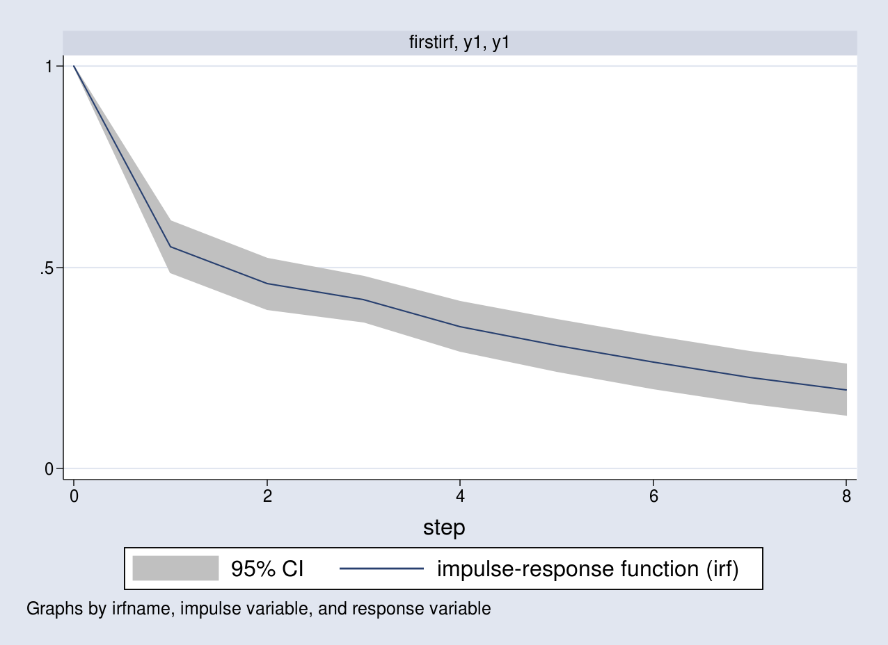
A unit impulse to the first equation increases y1 by a unit
contemporaneously. The response of y1 slowly declines over time to its long-run level.
Orthogonalized impulse–response functions
In the previous section, I showed the response of y1 due to a unit impulse on the same equation while holding the other impulse constant. The variance–covariance matrix \(\Sigmab\), however, implies a strong positive correlation between the two equations. I list the contents of the estimated variance–covariance matrix by typing
. matrix list e(Sigma)

symmetric e(Sigma)[2,2]
           y1         y2
y1  1.3055041
y2   .4639629  .74551376
The estimated covariance of the two equations is positive. This implies that I cannot assume the other impulse will remain constant. An impulse to the y2 equation has a contemporaneous effect on y1, and vice versa.
Orthogonalized impulse-response functions (OIRF) address this by decomposing the estimated variance–covariance matrix \(\hat{\Sigmab}\) into a lower triangular matrix. This type of decomposition isolates the contemporaneous response of y1 arising solely because of an impulse in the same equation. Nonetheless, the impulse on the first equation will still contemporaneously affect y2. For example, if y1 is inflation and y2 is interest rate, this decomposition implies that shock to inflation affects both inflation and interest rates. However, a shock to the interest rate equation only affects interest rates.
To estimate the OIRFs, let \({\bf P}\) denote the Cholesky decomposition of \(\Sigmab\) such that \({\bf P} {\bf P}’=\Sigmab\). Let \({\bf u}_t\) denote a \(2\times 1\) vector such that \({\bf P u}_t = \epsb_t\), which also implies \({\bf
u}_t = {\bf P}^{-1} \epsb_t\). The errors in \({\bf u}_t\) are uncorrelated by construction because \(E({\bf u}_t{\bf u}_t’) = {\bf P}^{-1}E(\epsb_t \epsb_t’) {\bf P’}^{-1}={\bf I}_2\). This allows us to interpret the OIRFs as a one standard-deviation impulse to \({\bf u}_t\).
I rewrite the MA(\(\infty\)) representation from earlier in terms of the \({\bf u}_t\) vector as
\[
{\bf y}_t = \sum_{p=0}^\infty \Phib_p \mub + \sum_{p=0}^\infty \Phib_p {\bf P u}_{t-p}
\]
The OIRFs are simply
\[
\frac{\partial y_{i,t+h}}{\partial u_{j,t}} = \{\Phib_h {\bf
P}\}_{i,j}
\]
the product of the MA coefficient matrices and the lower triangular matrix P.
I obtain the estimate of \(\Phat\) by typing
. matrix Sigma_hat = e(Sigma)

. matrix P_hat = cholesky(Sigma_hat)

. matrix list P_hat

P_hat[2,2]
           y1         y2
y1  1.1425866          0
y2  .40606367  .76198823
Using this matrix, I compute the first few responses as follows:
\begin{align*}
\begin{bmatrix} y_{1,0} \\ y_{2,0} \end{bmatrix} &=
\Phib_0 \Phat = {\bf I}_2 \Phat =
\begin{bmatrix} 1.1426 & 0\\ 0.4061 & 0.7620 \end{bmatrix} \\
\begin{bmatrix} y_{1,1} \\ y_{2,1} \end{bmatrix} &=
\hat{\Phib}_1 \Phat = \hat{{\bf A}}_1 \Phat =
\begin{bmatrix} 0.5046 & -0.2348 \\ 0.5234 & 0.1482 \end{bmatrix} \\
\begin{bmatrix} y_{1,2} \\ y_{2,2} \end{bmatrix} &= \hat{\Phib}_2 \Phat
= (\hat{{\bf A}}_1^2 + \hat{{\bf A}}_2) \Phat =
\begin{bmatrix} 0.5346 & 0.0194 \\ 0.2950 & -0.0275 \end{bmatrix}
\end{align*}
I list all the OIRFs in a table and plot the response of y1 due to an impulse in y1.
. irf table oirf, noci

                 Results from firstirf

+--------------------------------------------------------+
|        |    (1)    |    (2)    |    (3)    |    (4)    |
|  step  |   oirf    |   oirf    |   oirf    |   oirf    |
|--------+-----------+-----------+-----------+-----------|
|0       | 1.14259   | .406064   | 0         | .761988   |
|1       | .504552   | .523448   | -.23476   | .148171   |
|2       | .534588   | .294977   | .019384   | -.027504  |
|3       | .476019   | .279771   | -.0076    | .013468   |
|4       | .398398   | .242961   | -.010024  | -.00197   |
|5       | .346978   | .206023   | -.003571  | -.003519  |
|6       | .299284   | .178623   | -.004143  | -.001973  |
|7       | .257878   | .154023   | -.003555  | -.002089  |
|8       | .222533   | .13278    | -.002958  | -.001801  |
+--------------------------------------------------------+
(1) irfname = firstirf, impulse = y1, and response = y1
(2) irfname = firstirf, impulse = y1, and response = y2
(3) irfname = firstirf, impulse = y2, and response = y1
(4) irfname = firstirf, impulse = y2, and response = y2
irf table oirf requests the OIRFs. Notice that the estimates in the first three rows are the same as the ones computed above.
. irf graph oirf, impulse(y1) response(y1)
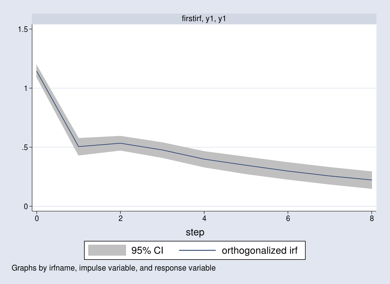
The graph corresponds to the response of y1 as a result of a one standard-deviation impulse to the same equation.
Conclusion
In this post, I showed how to simulate data from a stable VAR(2) model. I estimated the parameters of this model using the var command. I showed how to estimate IRFs and OIRFs. The latter obtains the responses using the lower triangular decomposition of the covariance matrix.
Reference
Lütkepohl, H. 2005. New Introduction to Multiple Time Series Analysis. New York: Springer.