Using the margins command with different functional forms: Proportional versus natural logarithm changes
margins is a powerful tool to obtain predictive margins, marginal predictions, and marginal effects. It is so powerful that it can work with any functional form of our estimated parameters by using the expression() option. I am going to show you how to obtain proportional changes of an outcome with respect to changes in the covariates using two different approaches for linear and nonlinear models.
Linear models with binary variables
After fitting a linear regression,
$$E(y|x) = a + b*x$$
we can estimate the proportional change of the fitted values with respect to a change in \(x\) (also known as, semielasticity) using margins, eydx(x). The formulas to estimate the semielasticity differ depending on whether \(x\) is continuous or discrete. If \(x\) is continuous,
\begin{equation}
{\bf eydx} = \frac{d({\rm ln}\widehat{y})}{dx}= \frac{dy}{dx}* \frac{1}{\widehat{y}} = \frac{\widehat{b}}{\widehat{y}}
\tag{1}
\end{equation}
When \(x\) is discrete, intuitively, we think the formula would be
\begin{equation}
{\bf eydx} = \frac{E(\widehat{y}|x = 1) – E(\widehat{y} |x = 0)}{E(\widehat{y}|x = 0)}\tag{2}
\end{equation}
However, this is not exactly what margins, eydx(x) calculates. Instead, margins obtains the difference of \(\widehat{y}\) relative to the base in the natural logarithm form,
\begin{equation}
{\bf eydx} = E\{{\rm ln}(\widehat{y})|x = 1\} – E\{{\rm ln}(\widehat{y})|x = 0\}\tag{3}
\end{equation}
To see an example, let’s fit our model with a continuous and a binary variable.
. webuse lbw, clear
(Hosmer & Lemeshow data)

. quietly regress bwt age i.ui

. margins, eydx(age ui)

Average marginal effects                                   Number of obs = 189
Model VCE: OLS

Expression: Linear prediction, predict()
ey/dx wrt:  age 1.ui

------------------------------------------------------------------------------
             |            Delta-method
             |      ey/dx   std. err.      t    P>|t|     [95% conf. interval]
-------------+----------------------------------------------------------------
         age |    .003225    .003309     0.97   0.331     -.003303    .0097531
        1.ui |  -.2082485   .0570519    -3.65   0.000    -.3208005   -.0956964
------------------------------------------------------------------------------
Note: ey/dx for factor levels is the discrete change from the base level.
We regressed babies’ birthweights (bwt) against mothers’ age (age) and the presence of uterine irritability (ui), where age is continuous and ui is a binary variable; then we computed semielasticities. We can manually calculate the proportional changes. The proportional change of the fitted value of bwt with respect to a change in age should be calculated as _b[age]/\(\widehat{{\bf bwt}}\), where _b[age] is the coefficient estimated for age and \(\widehat{{\bf bwt}}\) is the prediction for bwt.
. generate propage = _b[age]/(_b[_cons] + _b[age]*age + _b[1.ui]*ui)

. summarize propage

    Variable |        Obs        Mean    Std. dev.       Min        Max
-------------+---------------------------------------------------------
     propage |        189     .003225    .0002682   .0029186   .0039631
The reported mean, 0.003225, matches the semielasticity that margins yielded. We calculated the prediction of bwt using the generate command, but the prediction could more easily have been obtained by using the predict command. In the output of margins, we saw Expression: Linear prediction, predict() because in this case margins operates on the linear prediction. The expression can be changed and specified using the expression() option.
Let’s move on to ui, the proportional change of bwt with respect to a change in ui, based on (2),
$$\frac{\widehat{{\bf bwt}}|({\bf ui} = 1)-\widehat{{\bf bwt}}|({\bf ui} = 0)}{\widehat{{\bf bwt}}|({\bf ui} = 0)}$$
. preserve

. replace ui = 0
(28 real changes made)

. predict bwthat0
(option xb assumed; fitted values)

. replace ui = 1
(189 real changes made)

. predict bwthat1
(option xb assumed; fitted values)

. generate propui = (bwthat1 - bwthat0)/bwthat0

. summarize propui

    Variable |        Obs        Mean    Std. dev.       Min        Max
-------------+---------------------------------------------------------
      propui |        189    -.187989    .0030706  -.1935099  -.1760018
This time, \(-0.187989\) does not match the semielasticity reported by margins, \(-0.2082485\). As we already know, margins, eydx() does not calculate the proportional change with respect to a change in the categorical variable using (2). Instead, margins, eydx() replaces the derivative on the right-hand side of (1) with a change from the base level of the log of \(y\) [see (3)]. Let’s verify this in our example:
. generate lnbwt0  = ln(bwthat0)

. generate lnbwt1  = ln(bwthat1)

. generate propui2 = lnbwt1 - lnbwt0

. summarize propui2

    Variable |        Obs        Mean    Std. dev.       Min        Max
-------------+---------------------------------------------------------
     propui2 |        189   -.2082484    .0037771  -.2150636  -.1935868

. restore
margins, eydx() uses a method based on logs because this method has better numerical properties. In addition, if we have a model with the natural log of \(y\) on the left-hand side, then expressing the derivative with respect to the categorical variable as the difference from a base category is a common way of computing the proportional change. Suppose we have a model:
$$E\{{\rm ln}(y)\} = a + b*x$$
If variable x is categorical, then \(E({\rm ln}(y)|x = 1) – E({\rm ln}(y)|x = 0) = b\). There are cases when computing \(dy/dx*(1/y)\) differs from the change in the logs. This is true as we move away from models that have a logarithmic representation but even in these cases the approximation may be adequate if the proportional change in the outcome given a change in the covariate is small.
If we want to obtain the proportional change in (2) and its associated standard error, we can do this with margins, expression().
. margins, expression(_b[1.ui]/(_b[_cons] + _b[age]*age))
warning: option expression() does not contain option predict() or xb().

Predictive margins                                         Number of obs = 189
Model VCE: OLS

Expression: _b[1.ui]/(_b[_cons] + _b[age]*age)

------------------------------------------------------------------------------
             |            Delta-method
             |     Margin   std. err.      z    P>|z|     [95% conf. interval]
-------------+----------------------------------------------------------------
       _cons |   -.187989   .0463242    -4.06   0.000    -.2787827   -.0971952
------------------------------------------------------------------------------
In the expression() option, the denominator is the predicted bwt when ui = 0, and the numerator is the difference between the prediction of bwt when ui is 1 and when ui is 0. In the output of margins, the argument of expression() is specified after Expression:. The warning message cautions about the use of expression() without the predict() or xb() option. It is safe to ignore this message here. We will see examples demonstrating the use of these options in the Shortcuts in expression() option section.
Linear models with categorical variables
ui is a binary variable with values of 0 or 1. What if we have categorical variables with more than two groups? How can we use margins, expression() to compute a proportional change in this case? We would like to obtain the proportional change in the predicted outcome when the categorical variable changes from the base level to one of the other levels. Now, I am going to introduce the racial category variable (race =1 [White] 2 [Black] 3 [Other]) in the model, instead of uterine irritability.
. quietly regress bwt age i.race

. generate double propblack = _b[2.race]/(_b[_cons] + _b[age]*age)

. generate double propother = _b[3.race]/(_b[_cons] + _b[age]*age)

. summarize propblack propother

    Variable |        Obs        Mean    Std. dev.       Min        Max
-------------+---------------------------------------------------------
   propblack |        189   -.1183368    .0012359  -.1205344  -.1134239
   propother |        189   -.0927893    .0009691  -.0945124  -.0889371

. margins, expression((_b[2.race]*2.race + _b[3.race]*3.race)/
>                     (_b[_cons]+_b[age]*age)) dydx(race)
warning: option expression() does not contain option predict() or xb().

Average marginal effects                                   Number of obs = 189
Model VCE: OLS

Expression: (_b[2.race]*2.race + _b[3.race]*3.race)/ (_b[_cons]+_b[age]*age)
dy/dx wrt:  2.race 3.race

------------------------------------------------------------------------------
             |            Delta-method
             |      dy/dx   std. err.      z    P>|z|     [95% conf. interval]
-------------+----------------------------------------------------------------
        race |
      Black  |  -.1183368    .050575    -2.34   0.019    -.2174619   -.0192117
      Other  |  -.0927893   .0358962    -2.58   0.010    -.1631447    -.022434
------------------------------------------------------------------------------
Note: dy/dx for factor levels is the discrete change from the base level.
The manual calculations propblack and propother match what margins reported. Here I specified both the expression() and dydx() options. In the expression() option, the numerator includes the coefficient for each level of race (such as _b[2.race]) times the indicator for the observation belonging to the corresponding race (such as 2.race). The coefficient represents the difference between this race and the base category for race. After taking the derivative using dydx() with respect to each level,
\[
\frac{d({\bf expression})}{d({\bf 2.race})} = \frac{d\{({\bf \_b[2.race]*2.race} + {\bf \_b[3.race]*3.race})/({\bf \_b[\_cons]} + {\bf \_b[age]*age})\}}{d({\bf 2.race})}\\
\frac{d({\bf expression})}{d({\bf 3.race})} = \frac{d\{({\bf \_b[2.race]*2.race} + {\bf \_b[3.race]*3.race})/({\bf \_b[\_cons]} + {\bf \_b[age]*age})\}}{d({\bf 3.race})}
\]
we end up with the expressions of proportional changes with respect to Black and Other mothers,
$$
{\bf \_b[2.race]}/({\bf \_b[\_cons]} + {\bf \_b[age]*age}) \\
{\bf \_b[3.race]}/({\bf \_b[\_cons]} + {\bf \_b[age]*age})
$$
We could have instead used two separate margins, expression() commands to compute the proportional change for each group compared with the base, similar to what we did previously for the binary variable. Putting them in one expression makes it possible to further manipulate those margins. For instance, by estimating both proportional changes with one margins command, we now obtain both estimates along with the covariance of the estimates, and this allows us to test for a difference in the proportional changes.
Nonlinear models
The computations can be generalized to nonlinear models; the major difference would be the link function to compute the predicted outcome. In the next example, we use probit and Poisson regressions.
. quietly probit low age i.race

. margins, expression((normal(_b[_cons] + _b[age]*age
>                   + _b[2.race]*2.race + _b[3.race]*3.race)
>                   - normal(_b[_cons] + _b[age]*age))/
>                     normal(_b[_cons] + _b[age]*age)) dydx(race)
warning: option expression() does not contain option predict() or xb().

Average marginal effects                                   Number of obs = 189
Model VCE: OIM

Expression: (normal(_b[_cons] + _b[age]*age + _b[2.race]*2.race +
            _b[3.race]*3.race) - normal(_b[_cons] + _b[age]*age))/
            normal(_b[_cons] + _b[age]*age)
dy/dx wrt:  2.race 3.race

------------------------------------------------------------------------------
             |            Delta-method
             |      dy/dx   std. err.      z    P>|z|     [95% conf. interval]
-------------+----------------------------------------------------------------
        race |
      Black  |    .662603   .5016623     1.32   0.187    -.3206371    1.645843
      Other  |   .4874649   .3652971     1.33   0.182    -.2285042    1.203434
------------------------------------------------------------------------------
Note: dy/dx for factor levels is the discrete change from the base level.
In the probit regression, we modeled the probability of having a low-birthweight baby by using mothers’ age and racial categories. We obtained the proportional changes of predicted probability comparing Black with White mothers and Other with White mothers.
. webuse dollhill3, clear
(Doll and Hill (1966))

. quietly poisson deaths smokes i.agecat, exposure(pyears)

.  margins, expression((exp(_b[smokes]*smokes + _b[2.agecat]*2.agecat
>                    + _b[3.agecat]*3.agecat + _b[4.agecat]*4.agecat
>                    + _b[5.agecat]*5.agecat + _ b[_cons])*pyears
>                     - exp(_b[smokes]*smokes + _ b[_cons])*pyears)/
>                      (exp(_b[smokes]*smokes + _ b[_cons])*pyears))
>                       dydx(agecat)
warning: option expression() does not contain option predict() or xb().

Average marginal effects                                    Number of obs = 10
Model VCE: OIM

Expression: (exp(_b[smokes]*smokes + _b[2.agecat]*2.agecat +
            _b[3.agecat]*3.agecat + _b[4.agecat]*4.agecat +
            _b[5.agecat]*5.agecat + _ b[_cons])*pyears -
            exp(_b[smokes]*smokes + _ b[_cons])*pyears)/
            (exp(_b[smokes]*smokes + _ b[_cons])*pyears)
dy/dx wrt:  2.agecat 3.agecat 4.agecat 5.agecat

------------------------------------------------------------------------------
             |            Delta-method
             |      dy/dx   std. err.      z    P>|z|     [95% conf. interval]
-------------+----------------------------------------------------------------
      agecat |
      45–54  |   3.410584   .8605197     3.96   0.000     1.723996    5.097171
      55–64  |    12.8392   2.542638     5.05   0.000      7.85572    17.82268
      65–74  |   27.51678   5.269878     5.22   0.000     17.18801    37.84555
      75–84  |   39.45121   7.775511     5.07   0.000     24.21148    54.69093
------------------------------------------------------------------------------
Note: dy/dx for factor levels is the discrete change from the base level.
In the Poisson regression, the number of deaths was explained by smoking status and age category. The proportional changes of predicted number of deaths were computed by comparing each age group with the base.
margins operates on marginal prediction of the outcome, where the prediction equals xb in linear regression, equals \({\rm normal}(xb)\) in probit regression, and equals \({\rm exp}(xb) \times {\rm exposure}\) in Poisson regression. Furthermore, margins computes the prediction for each observation and reports the mean as the predictive margins.
Shortcuts in the expression() option
The functional forms we feed into margins, expression() can be as flexible and complex as needed. There are a few shortcuts that I would like to highlight here. Let’s go back to the probit regression.
. quietly probit low c.age##i.race

. margins, eydx(age)

Average marginal effects                                   Number of obs = 189
Model VCE: OIM

Expression: Pr(low), predict()
ey/dx wrt:  age

------------------------------------------------------------------------------
             |            Delta-method
             |      ey/dx   std. err.      z    P>|z|     [95% conf. interval]
-------------+----------------------------------------------------------------
         age |  -.0318742   .0234627    -1.36   0.174    -.0778603    .0141118
------------------------------------------------------------------------------
I introduced a two-way, full-factorial term between age and race. Here is the functional form spelled out to obtain margins, eydx(age):
\[
{\bf xb} = {\bf \_b[age]*age} + {\bf \_b[2.race\#c.age]*2.race*age} +{\bf \_b[3.race\#c.age]*3.race*age}
+ {\bf \_b[2.race]*2.race} + {\bf \_b[3.race]*3.race} + {\bf \_b[\_cons]} \\[.1in]
\frac{d {\rm ln}\{{\rm normal}(xb)\}}{d {\bf age}} =\frac{{\bf \_b[age]} + {\bf \_b[2.race\#c.age]*2.race} + {\bf \_b[3.race\#c.age]*3.race}}{{\rm normal}(xb)} \times {\rm normalden}(xb)
\]
In the expression() option, it is not necessary to write out the expression for things like linear prediction; thus, the above proportional change can be computed by
. margins, expression((_b[age] + _b[2.race#c.age]*2.race
>     + _b[3.race#c.age]*3.race)*normalden(predict(xb))/normal(predict(xb)
> ))

Predictive margins                                         Number of obs = 189
Model VCE: OIM

Expression: (_b[age] + _b[2.race#c.age]*2.race +
            _b[3.race#c.age]*3.race)*normalden(predict(xb))/
            > normal(predict(xb))

------------------------------------------------------------------------------
             |            Delta-method
             |     Margin   std. err.      z    P>|z|     [95% conf. interval]
-------------+----------------------------------------------------------------
       _cons |  -.0318742   .0234627    -1.36   0.174    -.0778603    .0141118
------------------------------------------------------------------------------
where predict(xb) is a shortcut to refer to the linear prediction. Further, normal(predict(xb)) can be replaced with predict(pr), where pr stands for probability of the positive outcome. The expression() option in margins lets us construct any functions of the estimated parameters and feed them back to margins. We then can use all the computations and graphical tools with marginsplot to visualize the result.
. quietly margins r.race, expression((_b[age] + _b[2.race#c.age]*2.race
>    + _b[3.race#c.age]*3.race)*normalden(predict(xb))/normal(predict(xb)))
>          at(age=(14(5)50))

. quietly marginsplot, noci ytitle("expression in -margins-")
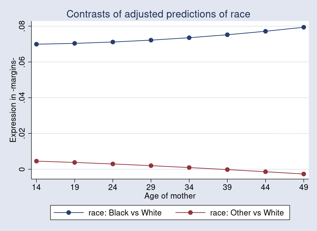
I obtained the proportional changes of predicted probability of having a low-birthweight baby with respect to the changes in mothers’ ages by comparing those from Black mothers and Other mothers with those from White mothers. The contrast is also visualized across a range of mothers’ ages from 14 through 50. The slightly diverging pattern might indicate the interaction effect that racial category moderates the relationship between the probability of having a low-birthweight baby and mothers’ age.
Conclusion
In this post, we learned how to use the expression() option with the margins command to obtain proportional changes of the outcome with respect to the changes in categorical covariates in both linear and nonlinear models. The expression() option is a versatile and powerful option that allows any functional form of estimated parameters and lets margins operate on the prediction of the outcome.