Bayesian threshold autoregressive models
Autoregressive (AR) models are some of the most widely used models in applied economics, among other disciplines, because of their generality and simplicity. However, the dynamic characteristics of real economic and financial data can change from one time period to another, limiting the applicability of linear time-series models. For example, the change of unemployment rate is a function of the state of the economy, whether it is expanding or contracting. A variety of models have been developed that allow time-series dynamics to depend on the regime of the system they are part of. The class of regime-dependent models include Markov-switching, smooth transition, and threshold autoregressive (TAR) models.
TAR (Tong 1982) is a class of nonlinear time-series models with applications in econometrics (Hansen 2011), financial analysis (Cao and Tsay 1992), and ecology (Tong 2011). TAR models allow regime-switching to be triggered by the observed level of an outcome in the past. The threshold command in Stata provides frequentist estimation of some TAR models.
In Stata 17, the bayesmh command supports time-series operators in linear and nonlinear model specifications; see [BAYES] bayesmh. In this blog entry, I want to show how we can fit some Bayesian TAR models using the bayesmh command. The examples will also demonstrate modeling flexibility not possible with the existing threshold command.
TAR model definition
Let \(\{y_t\}\) be a series observed at discrete times \(t\). A general TAR model of order \(p\), TAR(\(p\)), with \(k\) regimes has the form
\[
y_t = a_0^{j} + a_1^{j} y_{t-1} + \dots + a_p^{j} y_{t-p} + \sigma_{j} e_t, \quad {\rm if} \quad
r_{j-1} < z_t \le r_{j}
\]
where \(z_t\) is a threshold variable, \(-\infty < r_0 < \dots < r_k =
\infty\) are regime thresholds, and \(e_t\) are independent standard normally distributed errors. The \(j\)th regime has its own set of autoregressive coefficients \(\{a_i^j\}\)’s and standard deviations \(\sigma_j\)’s. Different regimes are also allowed to have different orders \(p\). In the above equation, this can be indicated by replacing \(p\) with regime-specific \(p_j\)’s.
In a TAR model, as implied by the definition, structural breaks happen not at certain time points but are triggered by the magnitude of the threshold variable \(z_t\). It is common to have \(z_t = y_{t-d}\), where \(d\) is a positive integer the called the delay parameter. These models are known as self-exciting TAR (SETAR) and are the ones I am illustrating below.
Real GDP dataset
In Beaudry and Koop (1993), TAR models were used to model gross national product. The authors demonstrated asymmetric persistence in the growth rate of gross national product, with positive shocks (associated with expansion periods) being more persistent than negative shocks (recession periods). In a similar approach, I use the growth rate of real gross domestic product (GDP) of the United States as an indicator of the status of the economy to model the difference between expansion and recession periods.
Quarterly observations on real GDP, measured in billions of dollars, are obtained from the Federal Reserve Economic Data repository using the import fred command. I consider observations only between the first quarter of 1947 and second quarter of 2021. A quarterly date variable, dateq, is generated and used with tsset to set up the time series.
. import fred GDPC1

Summary
-------------------------------------------------------------------------------
Series ID                    Nobs    Date range                Frequency
-------------------------------------------------------------------------------
GDPC1                        301     1947-01-01 to 2022-01-01  Quarterly
-------------------------------------------------------------------------------
# of series imported: 1
   highest frequency: Quarterly
    lowest frequency: Quarterly

. keep if daten >= date("01jan1947", "DMY") & daten <=
> date("01apr2021", "DMY")
(3 observations deleted)

. generate dateq = qofd(daten)

. tsset dateq, quarterly

Time variable: dateq, 1947q1 to 2021q2
        Delta: 1 quarter
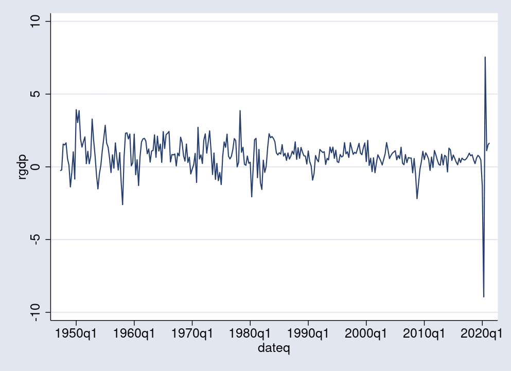
I am interested in the change of real GDP from one quarter to the next. For this purpose, I generate a new variable, rgdp, to measure this change in percentages. Positive values of rgdp indicate economic growth or expansion, while values close to 0 or negative are associated with stagnation or recession. Below, I use the tsline command to plot the time series. There, some of the recession periods, indicated by sharp drops in GDP, are visible, including the latest one in 2020.
. generate double rgdp = 100*D1.GDPC1/L1.GDPC1
(1 missing value generated)

. tsline rgdp
A TAR model with two regimes estimates one threshold value \(r\) that can be visualized as a horizontal line separating, somewhat informally, expansion from recession periods. In Bayesian TAR, the threshold \(r\) is a random variable with distribution estimated from a prior and observed data.
Bayesian TAR specification
Before I show how to specify a Bayesian TAR model in Stata, let me first fit a simpler Bayesian AR(1) model for rgdp using the bayesmh command. It will serve as a baseline for comparison with models with structural breaks.
I use the fairly uninformative, given the range of rgdp, normal(0, 100) prior for the two coefficients in the {rgdp:} equation and the igamma(0.01, 0.01) prior for the variance parameter {sig2}. I also use Gibbs sampling for more efficient simulation of the model parameters.
. bayesmh rgdp L1.rgdp, likelihood(normal({sig2}))
>         prior({rgdp:}, normal(0, 100)) block({rgdp:}, gibbs)
>         prior({sig2}, igamma(0.01, 0.01)) block({sig2}, gibbs)
>         rseed(17) dots

Burn-in 2500 .........1000.........2000..... done
Simulation 10000 .........1000.........2000.........3000.........4000.........
> 5000.........6000.........7000.........8000.........9000.........10000 done

Model summary
------------------------------------------------------------------------------
Likelihood:
  rgdp ~ normal(xb_rgdp,{sig2})

Priors:
  {rgdp:L.rgdp _cons} ~ normal(0,100)                                      (1)
               {sig2} ~ igamma(0.01,0.01)
------------------------------------------------------------------------------
(1) Parameters are elements of the linear form xb_rgdp.

Bayesian normal regression                       MCMC iterations  =     12,500
Gibbs sampling                                   Burn-in          =      2,500
                                                 MCMC sample size =     10,000
                                                 Number of obs    =        296
                                                 Acceptance rate  =          1
                                                 Efficiency:  min =      .9584
                                                              avg =      .9755
Log marginal-likelihood = -478.07327                          max =          1

------------------------------------------------------------------------------
             |                                                Equal-tailed
             |      Mean   Std. dev.     MCSE     Median  [95% cred. interval]
-------------+----------------------------------------------------------------
rgdp         |
        rgdp |
         L1. |  .1239926   .0579035   .000591   .1240375   .0096098    .237592
             |
       _cons |  .6762768   .0805277   .000805    .676687   .5186598   .8378632
-------------+----------------------------------------------------------------
        sig2 |  1.344712   .1098713   .001117   1.339746   1.144444   1.571802
------------------------------------------------------------------------------
The posterior mean estimate for the AR(1) coefficient {L1.rgdp} is 0.12, indicating a positive serial correlation for rgdp. This implies some degree of persistence in the real GDP growth. The posterior mean estimate of 1.34 for {sig2} suggests a volatility level above 1 percent, if the latter is measured by standard deviation. However, this simple AR(1) model does not tell us how the persistence and volatility change depending on the state of the economy.
Before continuing, I save the simulation and estimation results for later reference.
. bayesmh, saving(bar1sim, replace)
note: file bar1sim.dta saved.

. estimates store bar1
To describe a two-state model for the economy, I want to specify the simplest two-regime SETAR model with order of 1 and delay of 1. In the next section, I discuss the choice of order and delay parameters.
The model can be summarized by the following two equations:
\begin{align}
{\bf rgdp_t} = a_0^{1} + a_1^{1} {\bf rgdp_{t-1}} + \sigma_{1} e_t, \quad {\rm if} \quad
y_{t-1} < r \\
{\bf rgdp_t} = a_0^{2} + a_1^{2} {\bf rgdp_{t-1}} + \sigma_{2}
e_t, \quad {\rm if} \quad y_{t-1} \ge r
\end{align}
To specify the regression portion of this model with bayesmh, I use a substitutable expression with conditional logic,
cond(L1.rgdp<{r}, {r1:a0}+{r1:a1}*L1.rgdp, {r2:a0}+{r2:a1}*L1.rgdp)
where {r1:a0} and {r1:a1} are the coefficients for the first regime and {r2:a0} and {r2:a1} are the coefficients for the second regime.
The regime-specific variance of the normal likelihood can be similarly
specified by the expression
cond(L1.rgdp<{r},{sig1},{sig2})
Instead of assuming a fixed threshold value for \(r\), with 0 being a natural choice, I consider \(r\) to be a hyperparameter with uniform(-0.5, 0.5) prior. I thus assume that the threshold is within a half percentage point of 0. Given the range of rgdp and that 0 separates positive from negative growth, this seems to be a reasonable assumption. Using uninformative priors for \(r\) without any restrictions on its range will make the model unstable because of the possibility of collapsing one of the regimes, that is, having a regime with 0 or only a few observed points. The priors for coefficients and variances stay the same as in the previous model.
. bayesmh rgdp = (cond(L1.rgdp<{r},
>                 {r1:a0}+{r1:a1}*L1.rgdp,
>                 {r2:a0}+{r2:a1}*L1.rgdp)),
>         likelihood(normal(cond(L1.rgdp<{r}, {sig1}, {sig2})))
>         prior({r1:}, normal(0, 100)) block({r1:})
>         prior({r2:}, normal(0, 100)) block({r2:})
>         prior({sig1}, igamma(0.01, 0.01)) block({sig1})
>         prior({sig2}, igamma(0.01, 0.01)) block({sig2})
>         prior({r}, uniform(-0.5, 0.5)) block({r})
>         rseed(17) init({sig1} {sig2} 1) dots

Burn-in 2500 aaaaaaaaa1000aaaaaaaaa2000aaaaa done
Simulation 10000 .........1000.........2000.........3000.........4000.........
> 5000.........6000.........7000.........8000.........9000.........10000 done

Model summary
------------------------------------------------------------------------------
Likelihood:
  rgdp ~ normal(<expr1>,<expr2>)

Priors:
   {r1:a0 a1} ~ normal(0,100)
   {r2:a0 a1} ~ normal(0,100)
  {sig1 sig2} ~ igamma(0.01,0.01)
          {r} ~ uniform(-0.5,0.5)

Expressions:
  expr1 : cond(L1.rgdp<{r},{r1:a0}+{r1:a1}*L1.rgdp,{r2:a0}+{r2:a1}*L1.rgdp)
  expr2 : cond(L1.rgdp<{r},{sig1},{sig2})
------------------------------------------------------------------------------

Bayesian normal regression                       MCMC iterations  =     12,500
Random-walk Metropolis–Hastings sampling         Burn-in          =      2,500
                                                 MCMC sample size =     10,000
                                                 Number of obs    =        296
                                                 Acceptance rate  =      .3554
                                                 Efficiency:  min =     .04586
                                                              avg =      .1205
Log marginal-likelihood = -415.46111                          max =      .2235

------------------------------------------------------------------------------
             |                                                Equal-tailed
             |      Mean   Std. dev.     MCSE     Median  [95% cred. interval]
-------------+----------------------------------------------------------------
r1           |
          a0 | -1.327623   .7508926   .020208  -1.284013  -2.794005   .2010012
          a1 | -.8866186   .3328065   .009604  -.8828538  -1.582993  -.2458004
-------------+----------------------------------------------------------------
r2           |
          a0 |  .5521038   .0739373   .002338   .5516799   .4093326   .6992918
          a1 |  .3015663   .0555794   .001702   .3020909   .1883468   .4070365
-------------+----------------------------------------------------------------
           r | -.4834577   .0205573    .00096  -.4903714  -.4995296   -.416813
        sig1 |  6.752686   2.201104   .066593   6.356055   3.684466   12.27644
        sig2 |   .678672   .0580648   .001228    .676249   .5714164   .7989442
------------------------------------------------------------------------------
The model takes less than a minute to run. There are no obvious convergence problems reported by bayesmh, and the average sampling efficiency of 12% is good.
The threshold parameter is estimated to be about \(-0.48\). Although this is close to the lower limit of \(-0.5\) set by the prior, it is still strictly greater than \(-0.5\) because of its high precision—MCSE is less than 0.001.
The autoregression coefficients are negative in the first regime, r1, and positive in the second, r2. The second regime thus has much higher persistency. Also notable is the much higher variability in the first regime, about 6.75, in comparison with the second, 0.68.
I save the last estimation results and use the bayesstats ic command to compare the SETAR(1) and baseline AR(1) models.
. bayesmh, saving(bster1sim, replace)
note: file bster1sim.dta not found; file saved.

. estimates store bster1

. bayesstats ic bar1 bster1

Bayesian information criteria

----------------------------------------------
             |       DIC    log(ML)    log(BF)
-------------+--------------------------------
        bar1 |   929.311  -478.0733          .
      bster1 |  782.0817  -415.4611   62.61216
----------------------------------------------
Note: Marginal likelihood (ML) is computed
      using Laplace–Metropolis approximation.
The SETAR(1) model has a lower DIC and higher log-marginal likelihood than the AR(1) model. Of course, we expect the more complex and flexible SETAR(1) model to provide a better fit based on the likelihood alone. Note, however, that the marginal likelihood incorporates, in addition to the likelihood, the priors on model parameters and thus, indirectly, model complexity as well.
For comparison, I also perform frequentist estimation of the same model using the threshold command.
. threshold rgdp, regionvars(l.rgdp) threshvar(l1.rgdp)

Searching for threshold: 1
(running 237 regressions)
..................................................    50
..................................................   100
..................................................   150
..................................................   200
.....................................

Threshold regression
                                                       Number of obs =     296
Full sample: 1947q3 thru 2021q2                        AIC           = 30.1871
Number of thresholds = 1                               BIC           = 44.9485
Threshold variable: L.rgdp                             HQIC          = 36.0973

---------------------------------
Order     Threshold           SSR
---------------------------------
    1       -0.3881      319.0398
---------------------------------

------------------------------------------------------------------------------
        rgdp | Coefficient  Std. err.      z    P>|z|     [95% conf. interval]
-------------+----------------------------------------------------------------
Region1      |
        rgdp |
         L1. |  -.7989782     .12472    -6.41   0.000    -1.043425   -.5545315
             |
       _cons |  -.9796166   .2473612    -3.96   0.000    -1.464436   -.4947977
-------------+----------------------------------------------------------------
Region2      |
        rgdp |
         L1. |   .2910881   .0755517     3.85   0.000     .1430094    .4391667
             |
       _cons |   .5663334   .0987315     5.74   0.000     .3728231    .7598436
------------------------------------------------------------------------------
The estimates for regression coefficients are similar to the Bayesian ones: negative in the first regime and positive in the second regime. The threshold estimate is \(-0.39\), somewhat higher than the posterior mean estimate in the Bayesian model. A limitation of the threshold command is the lack of error-variance estimates for the two regimes.
Autoregression order selection
In the previous example, I fit the simplest SETAR model of order 1 and delay of 1. In general, these parameters are unknown, and one may not have a good prior choice for them. One solution is to fit models of different orders and compare them. A better solution is to consider one Bayesian model in which the orders are included as hyperparameters and are thus estimated along with all other parameters.
The following extension of the previous Bayesian model considers as possible choices orders from 1 to 4 for each regime. Two additional discrete hyperparameters, p1 and p2, indicate the regime orders. Both regimes are assumed to be at least of order 1. These hyperparameters thus take values in the set \(\{1,2,3,4\}\) according to some prior probabilities. I use the index(0.2,0.5,0.2,0.1) prior to set my highest expectation, 0.5, on order 2, then equal probabilities of 0.2 on orders 1 and 3, and finally probability of 0.1 on order 4. Orders 2, 3, and 4 are turned on and off using indicator variables as multipliers to the coefficients b2, b3, and b4, separately for each regime.
. bayesmh rgdp = (cond(L1.rgdp<{r},
>         {r1:a0} + {r1:a1}*L1.rgdp + ({p1}>1)*{r1:b2}*L2.rgdp +
>         ({p1}>2)*{r1:b3}*L3.rgdp  + ({p1}>3)*{r1:b4}*L4.rgdp,
>         {r2:a0} + {r2:a1}*L1.rgdp + ({p2}>1)*{r2:b2}*L2.rgdp +
>         ({p2}>2)*{r2:b3}*L3.rgdp  + ({p2}>3)*{r2:b4}*L4.rgdp)),
>         likelihood(normal(cond(L1.rgdp<{r}, {sig1}, {sig2})))
>         prior({p1}, index(0.2,0.5,0.2,0.1)) block({p1})
>         prior({p2}, index(0.2,0.5,0.2,0.1)) block({p2})
>         prior({r1:}, normal(0, 100)) block({r1:})
>         prior({r2:}, normal(0, 100)) block({r2:})
>         prior({sig1}, igamma(0.01, 0.01)) block({sig1})
>         prior({sig2}, igamma(0.01, 0.01)) block({sig2})
>         prior({r}, uniform(-0.5, 0.5)) block({r})
>         rseed(17) init({sig1} {sig2} 1 {p1} {p2} 2) dots

Burn-in 2500 aaaaaaaaa1000aaaaaaaaa2000aaaaa done
Simulation 10000 .........1000.........2000.........3000.........4000.........
> 5000.........6000.........7000.........8000.........9000.........10000 done

Model summary
------------------------------------------------------------------------------
Likelihood:
  rgdp ~ normal(<expr1>,<expr2>)

Priors:
              {p1 p2} ~ index(0.2,0.5,0.2,0.1)
  {r1:a0 a1 b2 b3 b4} ~ normal(0,100)
  {r2:a0 a1 b2 b3 b4} ~ normal(0,100)
          {sig1 sig2} ~ igamma(0.01,0.01)
                  {r} ~ uniform(-0.5,0.5)

Expressions:
  expr1 : cond(L1.rgdp<{r},{r1:a0} + {r1:a1}*L1.rgdp + ({p1}>1)*{r1:b2}*L2.rgd
          p + ({p1}>2)*{r1:b3}*L3.rgdp + ({p1}>3)*{r1:b4}*L4.rgdp,{r2:a0} +
          {r2:a1}*L1.rgdp + ({p2}>1)*{r2:b2}*L2.rgdp + ({p2}>2)*{r2:b3}*L3.rgd
          p + ({p2}>3)*{r2:b4}*L4.rgdp)
  expr2 : cond(L1.rgdp<{r},{sig1},{sig2})
------------------------------------------------------------------------------

Bayesian normal regression                       MCMC iterations  =     12,500
Random-walk Metropolis–Hastings sampling         Burn-in          =      2,500
                                                 MCMC sample size =     10,000
                                                 Number of obs    =        293
                                                 Acceptance rate  =      .3534
                                                 Efficiency:  min =      .0167
                                                              avg =     .04996
Log marginal-likelihood = -415.62492                          max =      .2163

------------------------------------------------------------------------------
             |                                                Equal-tailed
             |      Mean   Std. dev.     MCSE     Median  [95% cred. interval]
-------------+----------------------------------------------------------------
r1           |
          a0 | -1.382746   .7689649   .043474  -1.395605  -2.953167   .0933557
          a1 | -.8994067   .3164027   .021135  -.8966563   -1.53448  -.2834772
          b2 | -.6850185    8.58136   .561206   .0350022  -18.77976   16.92638
          b3 | -1.115146    9.72345   .595084  -.5968546  -20.72936   17.06076
          b4 |  .1783556   10.30925   .572088  -.0286035  -18.84217   21.22304
-------------+----------------------------------------------------------------
r2           |
          a0 |  .4381789   .0809618   .003256   .4369241   .2837359   .6029897
          a1 |  .3064629   .0549879   .002723   .3078107   .1969199    .409214
          b2 |  .1311621   .0531822   .004115   .1343153   .0269019   .2253627
          b3 | -.2968566   9.603545   .515804  -.1204644  -19.08613   18.83395
          b4 | -.9700926   9.811401   .462162  -1.123427  -20.09342   18.72596
-------------+----------------------------------------------------------------
          p1 |    1.1602   .3812486   .018329          1          1          2
          p2 |    1.9858   .1902682   .012683          2          1          2
           r | -.4845632   .0183435   .000932  -.4903276  -.4994973  -.4211905
        sig1 |  6.850306   2.403665   .078689   6.427896   3.629047   12.61115
        sig2 |  .6557395   .0570403   .001226   .6538532   .5533153   .7733018
------------------------------------------------------------------------------
The model takes about 2 minutes to run and has a good average sampling efficiency of 5%. Posterior median estimates for the order parameters are 1 for the first regime and 2 for the second. We saw that the first regime is more volatile. During recessions, having shorter order is consistent with having higher volatility.
Note that the parameters b2, b3, and b4 are not the actual autocorrelation coefficients for the series. To summarize the autoregression coefficients for the first regime, r1, we need to include the order indicators for p1 from the model specification.
. bayesstats summary {r1:a0} {r1:a1} (a2:({p1}>1)*{r1:b2})
>         (a3:({p1}>2)*{r1:b3}) (a4:({p1}>3)*{r1:b4})

Posterior summary statistics                      MCMC sample size =    10,000

          a2 : ({p1}>1)*{r1:b2}
          a3 : ({p1}>2)*{r1:b3}
          a4 : ({p1}>3)*{r1:b4}

------------------------------------------------------------------------------
             |                                                Equal-tailed
             |      Mean   Std. dev.     MCSE     Median  [95% cred. interval]
-------------+----------------------------------------------------------------
r1           |
          a0 | -1.382746   .7689649   .043474  -1.395605  -2.953167   .0933557
          a1 | -.8994067   .3164027   .021135  -.8966563   -1.53448  -.2834772
-------------+----------------------------------------------------------------
          a2 |  .0517708   .2540154   .013244          0  -.2375046   .9287818
          a3 | -.0014845    .038323   .000658          0          0          0
          a4 |         0          0         0          0          0          0
------------------------------------------------------------------------------
The autocorrelation estimates for orders 2 through 4 are very close to 0, as we expect given that the estimate for p1 is 1.
Similarly, the autoregression coefficients for the second regime have essentially estimates of 0 for orders 3 and 4.
. bayesstats summary {r2:a0} {r2:a1} (a2:({p2}>1)*{r2:b2})
>         (a3:({p2}>2)*{r2:b3}) (a4:({p2}>3)*{r2:b4})

Posterior summary statistics                      MCMC sample size =    10,000

          a2 : ({p2}>1)*{r2:b2}
          a3 : ({p2}>2)*{r2:b3}
          a4 : ({p2}>3)*{r2:b4}

------------------------------------------------------------------------------
             |                                                Equal-tailed
             |      Mean   Std. dev.     MCSE     Median  [95% cred. interval]
-------------+----------------------------------------------------------------
r2           |
          a0 |  .4381789   .0809618   .003256   .4369241   .2837359   .6029897
          a1 |  .3064629   .0549879   .002723   .3078107   .1969199    .409214
-------------+----------------------------------------------------------------
          a2 |  .1306131   .0480967   .003019   .1336667          0   .2179723
          a3 | -.0008258   .0089415   .000611          0          0          0
          a4 |         0          0         0          0          0          0
------------------------------------------------------------------------------
The delay \(d\) is another important parameter in SETAR models. Thus far, we considered a delay of one quarter period, which may not be optimal. Although it is possible to incorporate \(d\) as a hyperparameter in a single Bayesian model similarly to what I have done with the order parameters, to avoid an overly complicated specification, I run three additional models with \(d=2\), \(d=3\), and \(d=4\) by using L2.rgdp, L3.rgdp, and L4.rgdp, respectively, as threshold variables and compare them with the model with \(d=1\).
. bayesmh rgdp = (cond(L2.rgdp<{r},
>         {r1:a0} + {r1:a1}*L1.rgdp + ({p1}>1)*{r1:b2}*L2.rgdp +
>         ({p1}>2)*{r1:b3}*L3.rgdp  + ({p1}>3)*{r1:b4}*L4.rgdp,
>         {r2:a0} + {r2:a1}*L1.rgdp + ({p2}>1)*{r2:b2}*L2.rgdp +
>         ({p2}>2)*{r2:b3}*L3.rgdp  + ({p2}>3)*{r2:b4}*L4.rgdp)),
>         likelihood(normal(cond(L2.rgdp<{r}, {sig1}, {sig2})))
>         prior({p1}, index(0.2,0.5,0.2,0.1)) block({p1})
>         prior({p2}, index(0.2,0.5,0.2,0.1)) block({p2})
>         prior({r1:}, normal(0, 100)) block({r1:})
>         prior({r2:}, normal(0, 100)) block({r2:})
>         prior({sig1}, igamma(0.01, 0.01)) block({sig1})
>         prior({sig2}, igamma(0.01, 0.01)) block({sig2})
>         prior({r}, uniform(0, 1)) block({r})
>         rseed(17) init({sig1} {sig2} 1 {p1} {p2} 2)
>         burnin(5000) nomodelsummary notable

Burn-in ...
Simulation ...

Bayesian normal regression                       MCMC iterations  =     15,000
Random-walk Metropolis–Hastings sampling         Burn-in          =      5,000
                                                 MCMC sample size =     10,000
                                                 Number of obs    =        293
                                                 Acceptance rate  =      .3544
                                                 Efficiency:  min =     .01077
                                                              avg =     .05785
Log marginal-likelihood = -453.03074                          max =      .1904

. bayesmh rgdp = (cond(L3.rgdp<{r},
>         {r1:a0} + {r1:a1}*L1.rgdp + ({p1}>1)*{r1:b2}*L2.rgdp +
>         ({p1}>2)*{r1:b3}*L3.rgdp  + ({p1}>3)*{r1:b4}*L4.rgdp,
>         {r2:a0} + {r2:a1}*L1.rgdp + ({p2}>1)*{r2:b2}*L2.rgdp +
>         ({p2}>2)*{r2:b3}*L3.rgdp  + ({p2}>3)*{r2:b4}*L4.rgdp)),
>         likelihood(normal(cond(L3.rgdp<{r}, {sig1}, {sig2})))
>         prior({p1}, index(0.2,0.5,0.2,0.1)) block({p1})
>         prior({p2}, index(0.2,0.5,0.2,0.1)) block({p2})
>         prior({r1:}, normal(0, 100)) block({r1:})
>         prior({r2:}, normal(0, 100)) block({r2:})
>         prior({sig1}, igamma(0.01, 0.01)) block({sig1})
>         prior({sig2}, igamma(0.01, 0.01)) block({sig2})
>         prior({r}, uniform(0, 1)) block({r})
>         rseed(17) init({sig1} {sig2} 1 {p1} {p2} 2)
>         burnin(5000) nomodelsummary notable

Burn-in ...
Simulation ...

Bayesian normal regression                       MCMC iterations  =     15,000
Random-walk Metropolis–Hastings sampling         Burn-in          =      5,000
                                                 MCMC sample size =     10,000
                                                 Number of obs    =        293
                                                 Acceptance rate  =       .338
                                                 Efficiency:  min =    .006822
                                                              avg =      .0667
Log marginal-likelihood = -472.66834                          max =      .2068

. bayesmh rgdp = (cond(L4.rgdp<{r},
>         {r1:a0} + {r1:a1}*L1.rgdp + ({p1}>1)*{r1:b2}*L2.rgdp +
>         ({p1}>2)*{r1:b3}*L3.rgdp  + ({p1}>3)*{r1:b4}*L4.rgdp,
>         {r2:a0} + {r2:a1}*L1.rgdp + ({p2}>1)*{r2:b2}*L2.rgdp +
>         ({p2}>2)*{r2:b3}*L3.rgdp  + ({p2}>3)*{r2:b4}*L4.rgdp)),
>         likelihood(normal(cond(L4.rgdp<{r}, {sig1}, {sig2})))
>         prior({p1}, index(0.2,0.5,0.2,0.1)) block({p1})
>         prior({p2}, index(0.2,0.5,0.2,0.1)) block({p2})
>         prior({r1:}, normal(0, 100)) block({r1:})
>         prior({r2:}, normal(0, 100)) block({r2:})
>         prior({sig1}, igamma(0.01, 0.01)) block({sig1})
>         prior({sig2}, igamma(0.01, 0.01)) block({sig2})
>         prior({r}, uniform(0, 1)) block({r})
>         rseed(17) init({sig1} {sig2} 1 {p1} {p2} 2)
>         burnin(5000) nomodelsummary notable

Burn-in ...
Simulation ...

Bayesian normal regression                       MCMC iterations  =     15,000
Random-walk Metropolis–Hastings sampling         Burn-in          =      5,000
                                                 MCMC sample size =     10,000
                                                 Number of obs    =        293
                                                 Acceptance rate  =      .3749
                                                 Efficiency:  min =    .003091
                                                              avg =     .03948
Log marginal-likelihood = -484.88072                          max =      .1626
To save space, I show only the estimated log-marginal likelihoods of the models,
| \(d = 1\) | \(d = 2 \) | \(d = 3 \) | \(d = 4 \) |
| \(-416\) | \( -453 \) | \(-473 \) | \(-485 \) |
A delay of 1 gives us the highest log-marginal likelihood, thus validating our initial choice.
Final model
Here is our final model, which seems to provide the best analysis of the dynamics of rgdp.
. bayesmh rgdp = (cond(L1.rgdp<{r},
>                 {r1:a0}+{r1:a1}*L1.rgdp,
>                 {r2:a0}+{r2:a1}*L1.rgdp+{r2:a2}*L2.rgdp)),
>         likelihood(normal(cond(L1.rgdp<{r}, {sig1}, {sig2})))
>         prior({r1:}, normal(0, 100)) block({r1:})
>         prior({r2:}, normal(0, 100)) block({r2:})
>         prior({sig1}, igamma(0.01, 0.01)) block({sig1})
>         prior({sig2}, igamma(0.01, 0.01)) block({sig2})
>         prior({r}, uniform(-0.5, 0.5)) block({r})
>         rseed(17) init({sig1} {sig2} 1) dots

Burn-in 2500 aaaaaaaaa1000aaaaaaaaa2000aaaaa done
Simulation 10000 .........1000.........2000.........3000.........4000.........
> 5000.........6000.........7000.........8000.........9000.........10000 done

Model summary
------------------------------------------------------------------------------
Likelihood:
  rgdp ~ normal(<expr1>,<expr2>)

Priors:
     {r1:a0 a1} ~ normal(0,100)
  {r2:a0 a1 a2} ~ normal(0,100)
    {sig1 sig2} ~ igamma(0.01,0.01)
            {r} ~ uniform(-0.5,0.5)

Expressions:
  expr1 : cond(L1.rgdp<{r},{r1:a0}+{r1:a1}*L1.rgdp,{r2:a0}+{r2:a1}*
          L1.rgdp+{r2:a2}*L2.rgdp)
  expr2 : cond(L1.rgdp<{r},{sig1},{sig2})
------------------------------------------------------------------------------

Bayesian normal regression                       MCMC iterations  =     12,500
Random-walk Metropolis–Hastings sampling         Burn-in          =      2,500
                                                 MCMC sample size =     10,000
                                                 Number of obs    =        295
                                                 Acceptance rate  =      .3497
                                                 Efficiency:  min =     .04804
                                                              avg =     .09848
Log marginal-likelihood = -414.93784                          max =      .1997

------------------------------------------------------------------------------
             |                                                Equal-tailed
             |      Mean   Std. dev.     MCSE     Median  [95% cred. interval]
-------------+----------------------------------------------------------------
r1           |
          a0 | -1.269802   .7325285   .024046  -1.268012  -2.746194   .2098139
          a1 |  -.858765   .3224316   .009838  -.8566081   -1.48599  -.1966072
-------------+----------------------------------------------------------------
r2           |
          a0 |  .4496805   .0830125   .002535   .4501146   .2868064   .6120813
          a1 |  .2980119   .0562405   .001979   .2955394   .1915367    .412661
          a2 |  .1302317   .0417601   .001504   .1285035   .0465193   .2122086
-------------+----------------------------------------------------------------
           r | -.4831157   .0213086   .000972  -.4905123  -.4996558  -.4155153
        sig1 |  6.747231   2.396798   .087641   6.255731   3.666464    12.7075
        sig2 |  .6563023    .055926   .001251   .6510408   .5575998   .7745131
------------------------------------------------------------------------------
In conclusion, the expansion state, r2, is characterized by positive trend and autocorrelation, comparatively higher persistency, and lower volatility. The recession state, r1, on the other hand, experiences negative trend and autocorrelation, and higher volatility.
Although SETAR(1) provides a much more detailed analysis than a simple AR(1) model, it still does not capture all the changes in the dynamics of GDP growth. For example, the expansion periods before 1985 seem to have much higher volatility than those after 1985. Alternative regime-switching models may need to be considered to address this and other aspects of the time evolution of economic growth.
References
Beaudry, P., and G. Koop. 1993. Do recessions permanently change output? Journal of Monetary Economics 31: 149–163. https://doi.org/10.1016/0304-3932(93)90042-E.
Cao, C. Q., and R. S. Tsay. 1992. Nonlinear time-series analysis of stock volatilities. Journal of Applied Econometrics 7: S165–S185. https://doi.org/10.1002/jae.3950070512.
Hansen, B. E. 2011. Threshold autoregression in economics. Statistics and Its Inference 4: 123–127. https://doi.org/10.4310/SII.2011.v4.n2.a4.
Tong, H. 1982. Discontinuous decision processes and threshold autoregressive time series modelling. Biometrica 69: 274–276. https://doi.org/10.2307/2335885.
——. 2011. Threshold models in time series analysis—30 years on. Statistics and Its Inference 4: 107–118. https://dx.doi.org/10.4310/SII.2011.v4.n2.a1.