This post was written jointly with David Drukker, Director of Econometrics, StataCorp.

The topic for today is the treatment-effects features in Stata.

Treatment-effects estimators estimate the causal effect of a treatment on an outcome based on observational data.

In today’s posting, we will discuss four treatment-effects estimators:

1. RA: Regression adjustment
2. IPW: Inverse probability weighting
3. IPWRA: Inverse probability weighting with regression adjustment
4. AIPW: Augmented inverse probability weighting

We’ll save the matching estimators for part 2.

We should note that nothing about treatment-effects estimators magically extracts causal relationships. As with any regression analysis of observational data, the causal interpretation must be based on a reasonable underlying scientific rationale.

Introduction

We are going to discuss treatments and outcomes.

A treatment could be a new drug and the outcome blood pressure or cholesterol levels. A treatment could be a surgical procedure and the outcome patient mobility. A treatment could be a job training program and the outcome employment or wages. A treatment could even be an ad campaign designed to increase the sales of a product.

Consider whether a mother’s smoking affects the weight of her baby at birth. Questions like this one can only be answered using observational data. Experiments would be unethical.

The problem with observational data is that the subjects choose whether to get the treatment. For example, a mother decides to smoke or not to smoke. The subjects are said to have self-selected into the treated and untreated groups.

In an ideal world, we would design an experiment to test cause-and-effect and treatment-and-outcome relationships. We would randomly assign subjects to the treated or untreated groups. Randomly assigning the treatment guarantees that the treatment is independent of the outcome, which greatly simplifies the analysis.

Causal inference requires the estimation of the unconditional means of the outcomes for each treatment level. We only observe the outcome of each subject conditional on the received treatment regardless of whether the data are observational or experimental. For experimental data, random assignment of the treatment guarantees that the treatment is independent of the outcome; so averages of the outcomes conditional on observed treatment estimate the unconditional means of interest. For observational data, we model the treatment assignment process. If our model is correct, the treatment assignment process is considered as good as random conditional on the covariates in our model.

Let’s consider an example. Figure 1 is a scatterplot of observational data similar to those used by Cattaneo (2010). The treatment variable is the mother’s smoking status during pregnancy, and the outcome is the birthweight of her baby.

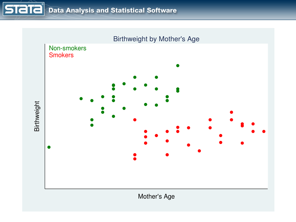
The red points represent the mothers who smoked during pregnancy, while the green points represent the mothers who did not. The mothers themselves chose whether to smoke, and that complicates the analysis.

We cannot estimate the effect of smoking on birthweight by comparing the mean birthweights of babies of mothers who did and did not smoke. Why not? Look again at our graph. Older mothers tend to have heavier babies regardless of whether they smoked while pregnant. In these data, older mothers were also more likely to be smokers. Thus, mother’s age is related to both treatment status and outcome. So how should we proceed?

RA: The regression adjustment estimator

RA estimators model the outcome to account for the nonrandom treatment assignment.

We might ask, “How would the outcomes have changed had the mothers who smoked chosen not to smoke?” or “How would the outcomes have changed had the mothers who didn’t smoke chosen to smoke?”. If we knew the answers to these counterfactual questions, analysis would be easy: we would just subtract the observed outcomes from the counterfactual outcomes.

The counterfactual outcomes are called unobserved potential outcomes in the treatment-effects literature. Sometimes the word unobserved is dropped.

We can construct measurements of these unobserved potential outcomes, and our data might look like this:

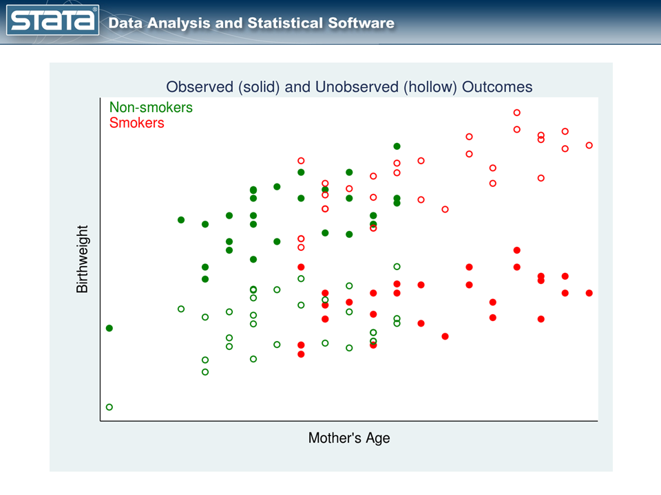
In figure 2, the observed data are shown using solid points and the unobserved potential outcomes are shown using hollow points. The hollow red points represent the potential outcomes for the smokers had they not smoked. The hollow green points represent the potential outcomes for the nonsmokers had they smoked.

We can estimate the unobserved potential outcomes then by fitting separate linear regression models with the observed data (solid points) to the two treatment groups.

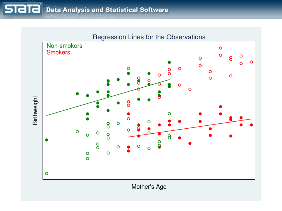
In figure 3, we have one regression line for nonsmokers (the green line) and a separate regression line for smokers (the red line).

Let’s understand what the two lines mean:

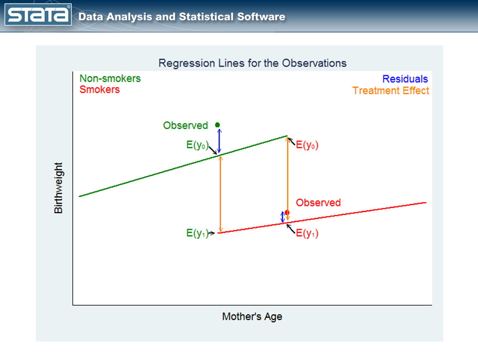
The green point on the left in figure 4, labeled Observed, is an observation for a mother who did not smoke. The point labeled E(y0) on the green regression line is the expected birthweight of the baby given the mother’s age and that she didn’t smoke. The point labeled E(y1) on the red regression line is the expected birthweight of the baby for the same mother had she smoked.

The difference between these expectations estimates the covariate-specific treatment effect for those who did not get the treatment.

Now, let’s look at the other counterfactual question.

The red point on the right in figure 4, labeled Observed in red, is an observation for a mother who smoked during pregnancy. The points on the green and red regression lines again represent the expected birthweights — the potential outcomes — of the mother’s baby under the two treatment conditions.

The difference between these expectations estimates the covariate-specific treatment effect for those who got the treatment.

Note that we estimate an average treatment effect (ATE), conditional on covariate values, for each subject. Furthermore, we estimate this effect for each subject, regardless of which treatment was actually received. Averages of these effects over all the subjects in the data estimate the ATE.

We could also use figure 4 to motivate a prediction of the outcome that each subject would obtain for each treatment level, regardless of the treatment recieved. The story is analogous to the one above. Averages of these predictions over all the subjects in the data estimate the potential-outcome means (POMs) for each treatment level.

It is reassuring that differences in the estimated POMs is the same estimate of the ATE discussed above.

The ATE on the treated (ATET) is like the ATE, but it uses only the subjects who were observed in the treatment group. This approach to calculating treatment effects is called regression adjustment (RA).

Let’s open a dataset and try this using Stata.

. webuse cattaneo2.dta, clear
(Excerpt from Cattaneo (2010) Journal of Econometrics 155: 138-154)

To estimate the POMs in the two treatment groups, we type

. teffects ra (bweight mage) (mbsmoke), pomeans

We specify the outcome model in the first set of parentheses with the outcome variable followed by its covariates. In this example, the outcome variable is bweight and the only covariate is mage.

We specify the treatment model — simply the treatment variable — in the second set of parentheses. In this example, we specify only the treatment variable mbsmoke. We’ll talk about covariates in the next section.

The result of typing the command is

. teffects ra (bweight mage) (mbsmoke), pomeans

Iteration 0:   EE criterion =  7.878e-24
Iteration 1:   EE criterion =  8.468e-26

Treatment-effects estimation                    Number of obs      =      4642
Estimator      : regression adjustment
Outcome model  : linear
Treatment model: none
------------------------------------------------------------------------------
             |               Robust
     bweight |      Coef.   Std. Err.      z    P>|z|     [95% Conf. Interval]
-------------+----------------------------------------------------------------
POmeans      |
     mbsmoke |
  nonsmoker  |   3409.435   9.294101   366.84   0.000     3391.219    3427.651
     smoker  |   3132.374   20.61936   151.91   0.000     3091.961    3172.787
------------------------------------------------------------------------------

The output reports that the average birthweight would be 3,132 grams if all mothers smoked and 3,409 grams if no mother smoked.

We can estimate the ATE of smoking on birthweight by subtracting the POMs: 3132.374 – 3409.435 = -277.061. Or we can reissue our teffects ra command with the ate option and get standard errors and confidence intervals:

. teffects ra (bweight mage) (mbsmoke), ate

Iteration 0:   EE criterion =  7.878e-24
Iteration 1:   EE criterion =  5.185e-26

Treatment-effects estimation                    Number of obs      =      4642
Estimator      : regression adjustment
Outcome model  : linear
Treatment model: none
-------------------------------------------------------------------------------
              |               Robust   
      bweight |      Coef.   Std. Err.      z    P>|z|     [95% Conf. Interval]
--------------+----------------------------------------------------------------
ATE           |        
      mbsmoke |
(smoker vs    |        
  nonsmoker)  |  -277.0611   22.62844   -12.24   0.000    -321.4121   -232.7102
--------------+----------------------------------------------------------------
POmean        |        
      mbsmoke |
   nonsmoker  |   3409.435   9.294101   366.84   0.000     3391.219    3427.651
-------------------------------------------------------------------------------

The output reports the same ATE we calculated by hand: -277.061. The ATE is the average of the differences between the birthweights when each mother smokes and the birthweights when no mother smokes.

We can also estimate the ATET by using the teffects ra command with option atet, but we will not do so here.

IPW: The inverse probability weighting estimator

RA estimators model the outcome to account for the nonrandom treatment assignment. Some researchers prefer to model the treatment assignment process and not specify a model for the outcome.

We know that smokers tend to be older than nonsmokers in our data. We also hypothesize that mother’s age directly affects birthweight. We observed this in figure 1, which we show again below.

This figure shows that treatment assignment depends on mother’s age. We would like to have a method of adjusting for this dependence. In particular, we wish we had more upper-age green points and lower-age red points. If we did, the mean birthweight for each group would change. We don’t know how that would affect the difference in means, but we do know it would be a better estimate of the difference.

To achieve a similar result, we are going to weight smokers in the lower-age range and nonsmokers in the upper-age range more heavily, and weight smokers in the upper-age range and nonsmokers in the lower-age range less heavily.

We will fit a probit or logit model of the form

Pr(woman smokes) = F(a + b*age)

teffects uses logit by default, but we will specify the probit option for illustration.

Once we have fit that model, we can obtain the prediction Pr(woman smokes) for each observation in the data; we’ll call this p_i. Then, in making our POMs calculations — which is just a mean calculation — we will use those probabilities to weight the observations. We will weight observations on smokers by 1/p_i so that weights will be large when the probability of being a smoker is small. We will weight observations on nonsmokers by 1/(1-p_i) so that weights will be large when the probability of being a nonsmoker is small.

That results in the following graph replacing figure 1:

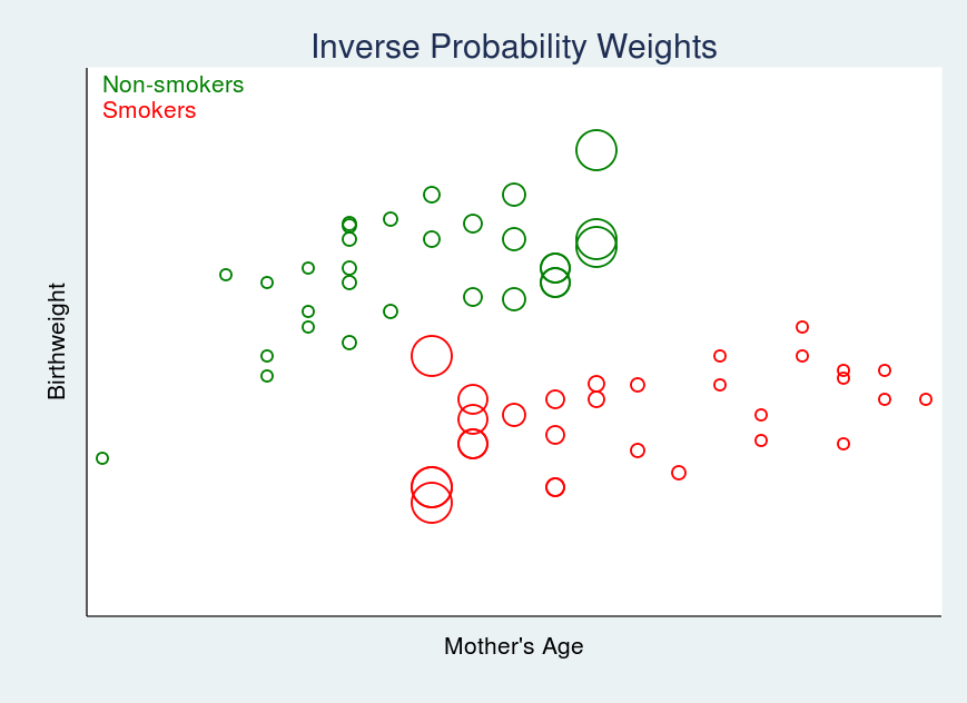
In figure 5, larger circles indicate larger weights.

To estimate the POMs with this IPW estimator, we can type

. teffects ipw (bweight) (mbsmoke mage, probit), pomeans

The first set of parentheses specifies the outcome model, which is simply the outcome variable in this case; there are no covariates. The second set of parentheses specifies the treatment model, which includes the outcome variable (mbsmoke) followed by covariates (in this case, just mage) and the kind of model (probit).

The result is

. teffects ipw (bweight) (mbsmoke mage, probit), pomeans

Iteration 0:   EE criterion =  3.615e-15
Iteration 1:   EE criterion =  4.381e-25

Treatment-effects estimation                    Number of obs      =      4642
Estimator      : inverse-probability weights
Outcome model  : weighted mean
Treatment model: probit
------------------------------------------------------------------------------
             |               Robust
     bweight |      Coef.   Std. Err.      z    P>|z|     [95% Conf. Interval]
-------------+----------------------------------------------------------------
POmeans      |
     mbsmoke |
  nonsmoker  |   3408.979   9.307838   366.25   0.000     3390.736    3427.222
     smoker  |   3133.479   20.66762   151.61   0.000     3092.971    3173.986
------------------------------------------------------------------------------

Our output reports that the average birthweight would be 3,133 grams if all the mothers smoked and 3,409 grams if none of the mothers smoked.

This time, the ATE is -275.5, and if we typed

. teffects ipw (bweight) (mbsmoke mage, probit), ate
(Output omitted)

we would learn that the standard error is 22.68 and the 95% confidence interval is [-319.9,231.0].

Just as with teffects ra, if we wanted ATET, we could specify the teffects ipw command with the atet option.

IPWRA: The IPW with regression adjustment estimator

RA estimators model the outcome to account for the nonrandom treatment assignment. IPW estimators model the treatment to account for the nonrandom treatment assignment. IPWRA estimators model both the outcome and the treatment to account for the nonrandom treatment assignment.

IPWRA uses IPW weights to estimate corrected regression coefficients that are subsequently used to perform regression adjustment.

The covariates in the outcome model and the treatment model do not have to be the same, and they often are not because the variables that influence a subject’s selection of treatment group are often different from the variables associated with the outcome. The IPWRA estimator has the double-robust property, which means that the estimates of the effects will be consistent if either the treatment model or the outcome model — but not both — are misspecified.

Let’s consider a situation with more complex outcome and treatment models but still using our low-birthweight data.

The outcome model will include

1. mage: the mother’s age
2. prenatal1: an indicator for prenatal visit during the first trimester
3. mmarried: an indicator for marital status of the mother
4. fbaby: an indicator for being first born

The treatment model will include

1. all the covariates of the outcome model
2. mage^2
3. medu: years of maternal education

We will also specify the aequations option to report the coefficients of the outcome and treatment models.

. teffects ipwra (bweight mage prenatal1 mmarried fbaby)                ///
                 (mbsmoke mmarried c.mage##c.mage fbaby medu, probit)   ///
                 , pomeans aequations

Iteration 0:   EE criterion =  1.001e-20
Iteration 1:   EE criterion =  1.134e-25

Treatment-effects estimation                    Number of obs      =      4642
Estimator      : IPW regression adjustment
Outcome model  : linear
Treatment model: probit
-------------------------------------------------------------------------------
              |               Robust
      bweight |      Coef.   Std. Err.      z    P>|z|     [95% Conf. Interval]
--------------+----------------------------------------------------------------
POmeans       |
      mbsmoke |
   nonsmoker  |   3403.336    9.57126   355.58   0.000     3384.576    3422.095
      smoker  |   3173.369   24.86997   127.60   0.000     3124.624    3222.113
--------------+----------------------------------------------------------------
OME0          |
         mage |   2.893051   2.134788     1.36   0.175    -1.291056    7.077158
    prenatal1 |   67.98549   28.78428     2.36   0.018     11.56933    124.4017
     mmarried |   155.5893   26.46903     5.88   0.000      103.711    207.4677
        fbaby |   -71.9215   20.39317    -3.53   0.000    -111.8914   -31.95162
        _cons |   3194.808   55.04911    58.04   0.000     3086.913    3302.702
--------------+----------------------------------------------------------------
OME1          |
         mage |  -5.068833   5.954425    -0.85   0.395    -16.73929    6.601626
    prenatal1 |   34.76923   43.18534     0.81   0.421    -49.87248    119.4109
     mmarried |   124.0941   40.29775     3.08   0.002     45.11193    203.0762
        fbaby |   39.89692   56.82072     0.70   0.483    -71.46966    151.2635
        _cons |   3175.551   153.8312    20.64   0.000     2874.047    3477.054
--------------+----------------------------------------------------------------
TME1          |
     mmarried |  -.6484821   .0554173   -11.70   0.000     -.757098   -.5398663
         mage |   .1744327   .0363718     4.80   0.000     .1031452    .2457202
              |
c.mage#c.mage |  -.0032559   .0006678    -4.88   0.000    -.0045647   -.0019471
              |
        fbaby |  -.2175962   .0495604    -4.39   0.000    -.3147328   -.1204595
         medu |  -.0863631   .0100148    -8.62   0.000    -.1059917   -.0667345
        _cons |  -1.558255   .4639691    -3.36   0.001    -2.467618   -.6488926
-------------------------------------------------------------------------------

The POmeans section of the output displays the POMs for the two treatment groups. The ATE is now calculated to be 3173.369 – 3403.336 = -229.967.

The OME0 and OME1 sections display the RA coefficients for the untreated and treated groups, respectively.

The TME1 section of the output displays the coefficients for the probit treatment model.

Just as in the two previous cases, if we wanted the ATE with standard errors, etc., we would specify the ate option. If we wanted ATET, we would specify the atet option.

AIPW: The augmented IPW estimator

IPWRA estimators model both the outcome and the treatment to account for the nonrandom treatment assignment. So do AIPW estimators.

The AIPW estimator adds a bias-correction term to the IPW estimator. If the treatment model is correctly specified, the bias-correction term is 0 and the model is reduced to the IPW estimator. If the treatment model is misspecified but the outcome model is correctly specified, the bias-correction term corrects the estimator. Thus, the bias-correction term gives the AIPW estimator the same double-robust property as the IPWRA estimator.

The syntax and output for the AIPW estimator is almost identical to that for the IPWRA estimator.

. teffects aipw (bweight mage prenatal1 mmarried fbaby)                 ///
                (mbsmoke mmarried c.mage##c.mage fbaby medu, probit)    ///
                , pomeans aequations

Iteration 0:   EE criterion =  4.632e-21
Iteration 1:   EE criterion =  5.810e-26

Treatment-effects estimation                    Number of obs      =      4642
Estimator      : augmented IPW
Outcome model  : linear by ML
Treatment model: probit
-------------------------------------------------------------------------------
              |               Robust
      bweight |      Coef.   Std. Err.      z    P>|z|     [95% Conf. Interval]
--------------+----------------------------------------------------------------
POmeans       |
      mbsmoke |
   nonsmoker  |   3403.355   9.568472   355.68   0.000     3384.601    3422.109
      smoker  |   3172.366   24.42456   129.88   0.000     3124.495    3220.237
--------------+----------------------------------------------------------------
OME0          |
         mage |   2.546828   2.084324     1.22   0.222    -1.538373    6.632028
    prenatal1 |   64.40859   27.52699     2.34   0.019     10.45669    118.3605
     mmarried |   160.9513    26.6162     6.05   0.000     108.7845    213.1181
        fbaby |   -71.3286   19.64701    -3.63   0.000     -109.836   -32.82117
        _cons |   3202.746   54.01082    59.30   0.000     3096.886    3308.605
--------------+----------------------------------------------------------------
OME1          |
         mage |  -7.370881    4.21817    -1.75   0.081    -15.63834    .8965804
    prenatal1 |   25.11133   40.37541     0.62   0.534    -54.02302    104.2457
     mmarried |   133.6617   40.86443     3.27   0.001      53.5689    213.7545
        fbaby |   41.43991   39.70712     1.04   0.297    -36.38461    119.2644
        _cons |   3227.169   104.4059    30.91   0.000     3022.537    3431.801
--------------+----------------------------------------------------------------
TME1          |
     mmarried |  -.6484821   .0554173   -11.70   0.000     -.757098   -.5398663
         mage |   .1744327   .0363718     4.80   0.000     .1031452    .2457202
              |
c.mage#c.mage |  -.0032559   .0006678    -4.88   0.000    -.0045647   -.0019471
              |
        fbaby |  -.2175962   .0495604    -4.39   0.000    -.3147328   -.1204595
         medu |  -.0863631   .0100148    -8.62   0.000    -.1059917   -.0667345
        _cons |  -1.558255   .4639691    -3.36   0.001    -2.467618   -.6488926
-------------------------------------------------------------------------------

The ATE is 3172.366 – 3403.355 = -230.989.

Final thoughts

The example above used a continuous outcome: birthweight. teffects can also be used with binary, count, and nonnegative continuous outcomes.

The estimators also allow multiple treatment categories.

An entire manual is devoted to the treatment-effects features in Stata 13, and it includes a basic introduction, advanced discussion, and worked examples. If you would like to learn more, you can download the [TE] Treatment-effects Reference Manual from the Stata website.

More to come

Next time, in part 2, we will cover the matching estimators.

Reference

Cattaneo, M. D. 2010. Efficient semiparametric estimation of multi-valued treatment effects under ignorability. Journal of Econometrics 155: 138–154.