Programming an estimation command in Stata: Where to store your stuff
If you tell me “I program in Stata”, it makes me happy, but I do not know what you mean. Do you write scripts to make your research reproducible, or do you write Stata commands that anyone can use and reuse? In the series #StataProgramming, I will show you how to write your own commands, but I start at the beginning. Discussing the difference between scripts and commands here introduces some essential programming concepts and constructions that I use to write scripts and commands.
This is the second post in the series Programming an estimation command in Stata. I recommend that you start at the beginning. See Programming an estimation command in Stata: A map to posted entries for a map to all the posts in this series.
Scripts versus commands
A script is a program that always performs the same tasks on the same inputs and produces exactly the same results. Scripts in Stata are known as do-files and the files containing them end in .do. For example, I could write a do-file to
- read in the National Longitudinal Study of Youth (NLSY) dataset,
- clean the data,
- form a sample for some population, and
- run a bunch of regressions on the sample.
This structure is at the heart of reproducible research; produce the same results from the same inputs every time. Do-files have a one-of structure. For example, I could not somehow tell this do-file that I want it to perform the analogous tasks on the Panel Study on Income Dynamics (PSID). Commands are reusable programs that take arguments to perform a task on any data of certain type. For example, regress performs ordinary least squares on the specified variables regardless of whether they come from the NLSY, PSID, or any other dataset. Stata commands are written in the automatic do-file (ado) language; the files containing them end in .ado. Stata commands written in the ado language are known as ado-commands.
An example do-file
The commands in code block 1 are contained in the file doex.do in the current working directory of my computer.
// version 1.0.0  04Oct2015 (This line is comment)
version 14                     // version #.# fixes the version of Stata
use http://www.stata.com/data/accident2.dta
summarize accidents tickets
We execute the commands by typing do doex which produces
Example 1: Output from do doex
. do doex

. // version 1.0.0  04Oct2015 (This line is comment)
. version 14                     // version #.# fixes the version of Stata

. use http://www.stata.com/data/accident2.dta

. summarize accidents tickets

    Variable |        Obs        Mean    Std. Dev.       Min        Max
-------------+---------------------------------------------------------
   accidents |        948    .8512658    2.851856          0         20
     tickets |        948    1.436709    1.849456          0          7

.
.
end of do-file
- Line 1 in doex.do is a comment that helps to document the code but is not executed by Stata. The // initiates a comment. Anything following the // on that line is ignored by Stata.
- In the comment on line 1, I put a version number and the date that I last changed this file. The date and the version help me keep track of the changes that I make as I work on the project. This information also helps me answer questions from others with whom I have shared a version of this file.
- Line 2 specifies the definition of the Stata language that I use. Stata changes over time. Setting the version ensures that the do-file continues to run and that the results do not change as the Stata language evolves.
- Line 3 reads in the accident.dta dataset.
- Line 4 summarizes the variables accidents and tickets.
Storing stuff in Stata
Programming in Stata is like putting stuff into boxes, making Stata change the stuff in the boxes, and getting the changed stuff out of the boxes. For example, code block 2 contains the code for doex2.do, whose output I display in example 2
// version 1.0.0  04Oct2015 (This line is comment)
version 14                     // version #.# fixes the version of Stata
use http://www.stata.com/data/accident2.dta
generate ln_traffic = ln(traffic)
summarize ln_traffic
Example 2: Output from do doex2
. do doex2

. // version 1.0.0  04Oct2015 (This line is comment)
. version 14                     // version #.# fixes the version of Stata

. use http://www.stata.com/data/accident2.dta

. generate ln_traffic = ln(traffic)

. summarize ln_traffic

    Variable |        Obs        Mean    Std. Dev.       Min        Max
-------------+---------------------------------------------------------
  ln_traffic |        948    1.346907    1.004952  -5.261297   2.302408

.
.
end of do-file
In line 4 of code block 2, I generate the new variable ln_traffic which I summarize on line 5. doex2.do uses generate to change what is in the box ln_traffic and uses summarize to get a function of the changed stuff out of the box. Stata variables are the most frequently used box type in Stata, but when you are programming, you will also rely on Stata matrices.
There can only be one variable named traffic in a Stata dataset and its contents can be viewed or changed interactively, by a do-file, or by an ado-file command. Similarly, there can only be one Stata matrix named beta in a Stata session and its contents can be viewed or changed interactively, by a do-file, or by an ado-file command. Stata variables and Stata matrices are global boxes because there can only be one Stata variable or Stata matrix in a Stata session and its contents can be viewed or changed anywhere in a Stata session.
The opposite of global is local. If it is local in Stata, its contents can only be accessed or changed in the interactive session, in a particular do-file, or a in particular ado-file.
Although I am discussing do-files at the moment, remember that we are learning techniques to write commands. It is essential to understand the differences between global boxes and local boxes to program commands in Stata. Global boxes, like variables, could contain data that the users of your command do not want changed. For example, a command you write should never change a user’s variable in a way that was not requested.
Levels of Stata
The notion that there are levels of Stata can help explain the difference between global boxes and local boxes. Suppose that I run 2 do-files or ado-files. Think of the interactive Stata session as level 0 of Stata, and think of each do-file or ado-file as being Stata levels 1 and 2. Global boxes like variables and matrices live in global memory that can be accessed or changed from a Stata command executed in level 0, 1, or 2. Local boxes can only be accessed or changed by a Stata command within a particular level of Stata. (This description is not exactly how Stata works, but the details about how Stata really handles levels are not important here.)
Figure 1 depicts this structure.
Memory by Stata level
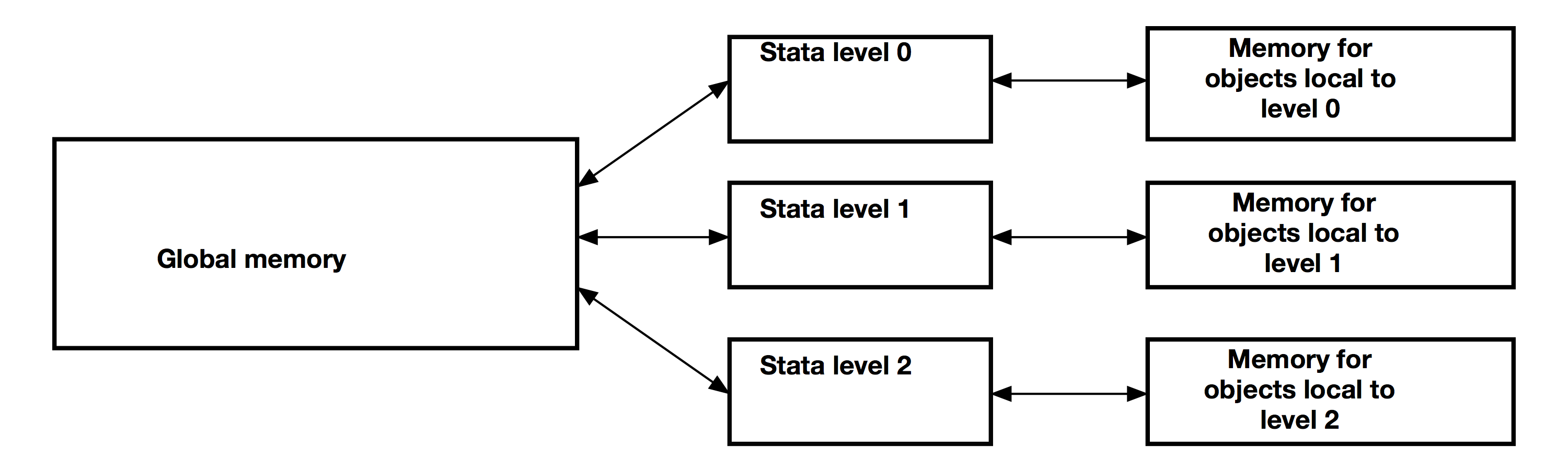
Figure 1 clarifies
- that commands executed at all Stata levels can access and change the objects in global memory,
- that only commands executed at Stata level 0 can access and change the objects local to Stata level 0,
- that only commands executed at Stata level 1 can access and change the objects local to Stata level 1, and
- that only commands executed at Stata level 2 can access and change the objects local to Stata level 2.
Global and local macros: Storing and extracting
Macros are Stata boxes that hold information as characters, also known as strings. Stata has both global macros and local macros. Global macros are global and local macros are local. Global macros can be accessed and changed by a command executed at any Stata level. Local macros can be accessed and changed only by a command executed at a specific Stata level.
The easiest way to begin to understand global macros is to put something into a global macro and then to get it back out. Code block 3 contains the code for global1.do which stores and the retrieves information from a global macro.
// version 1.0.0  04Oct2015
version 14
global vlist "y x1 x2"
display "vlist contains $vlist"
Example 3: Output from do global1
. do global1

. // version 1.0.0  04Oct2015
. version 14

. global vlist "y x1 x2"

. display "vlist contains $vlist"
vlist contains y x1 x2

.
end of do-file
Line 3 of code block 3 puts the string y x1 x2 into the global macro named vlist. To extract what I put into a global macro, I prefix the name of global macro with a $. Line 4 of the code block and its output in example 3 illustrate this usage by extracting and displaying the contents of vlist.
Code block 4 contains the code for local1.do and its output is given in example 4. They illustrate how to put something into a local macro and how to extract something from it.
// version 1.0.0  04Oct2015
version 14
local vlist "y x1 x2"
display "vlist contains `vlist'"
Example 4: Output from do global1
. do local1

. // version 1.0.0  04Oct2015
. version 14

. local vlist "y x1 x2"

. display "vlist contains `vlist'"
vlist contains y x1 x2

.
end of do-file
Line 3 of code block 3 puts the string y x1 x2 into the local macro named vlist. To extract what I put into a local macro I enclose the name of the local macro between a single left quote (‘) and a single right quote (’). Line 4 of code block 3 displays what is contained in the local macro vlist and its output in example 4 illustrates this usage.
Getting stuff from Stata commands
Now that we have boxes, I will show you how to store stuff computed by Stata in these boxes. Analysis commands, like summarize, store their results in r(). Estimation commands, like regress, store their results in e(). Somewhat tautologically, commands that store their results in r() are also known as r-class commands and commands that store their results in e() are also known as e-class commands.
I can use return list to see results stored by an r-class command. Below, I list out what summarize has stored in r() and compute the mean from the stored results.
Example 5: Getting results from an r-class command
. use http://www.stata.com/data/accident2.dta, clear

. summarize accidents

    Variable |        Obs        Mean    Std. Dev.       Min        Max
-------------+---------------------------------------------------------
   accidents |        948    .8512658    2.851856          0         20

. return list

scalars:
                  r(N) =  948
              r(sum_w) =  948
               r(mean) =  .8512658227848101
                r(Var) =  8.133081817331211
                 r(sd) =  2.851855854935732
                r(min) =  0
                r(max) =  20
                r(sum) =  807

. local sum = r(sum)

. local N   = r(N)

. display "The mean is " `sum'/`N'
The mean is .85126582
Estimation commands are more formal than analysis commands, so they save more stuff.
Official Stata estimation commands save lots of stuff, because they follow lots of rules that make postestimation easy for users. Do not be alarmed by the number of things stored by poisson. Below, I list out the results stored by poisson and create a Stata matrix that contains the coefficient estimates.
Example 6: Getting results from an e-class command
. poisson accidents traffic tickets male

Iteration 0:   log likelihood = -377.98594
Iteration 1:   log likelihood = -370.68001
Iteration 2:   log likelihood = -370.66527
Iteration 3:   log likelihood = -370.66527

Poisson regression                              Number of obs     =        948
                                                LR chi2(3)        =    3357.64
                                                Prob > chi2       =     0.0000
Log likelihood = -370.66527                     Pseudo R2         =     0.8191

------------------------------------------------------------------------------
   accidents |      Coef.   Std. Err.      z    P>|z|     [95% Conf. Interval]
-------------+----------------------------------------------------------------
     traffic |   .0764399   .0129856     5.89   0.000     .0509887    .1018912
     tickets |   1.366614   .0380641    35.90   0.000      1.29201    1.441218
        male |   3.228004   .1145458    28.18   0.000     3.003499     3.45251
       _cons |  -7.434478   .2590086   -28.70   0.000    -7.942126    -6.92683
------------------------------------------------------------------------------

. ereturn list

scalars:
               e(rank) =  4
                  e(N) =  948
                 e(ic) =  3
                  e(k) =  4
               e(k_eq) =  1
               e(k_dv) =  1
          e(converged) =  1
                 e(rc) =  0
                 e(ll) =  -370.6652697757637
         e(k_eq_model) =  1
               e(ll_0) =  -2049.485325326086
               e(df_m) =  3
               e(chi2) =  3357.640111100644
                  e(p) =  0
               e(r2_p) =  .8191422669899876

macros:
            e(cmdline) : "poisson accidents traffic tickets male"
                e(cmd) : "poisson"
            e(predict) : "poisso_p"
          e(estat_cmd) : "poisson_estat"
           e(chi2type) : "LR"
                e(opt) : "moptimize"
                e(vce) : "oim"
              e(title) : "Poisson regression"
               e(user) : "poiss_lf"
          e(ml_method) : "e2"
          e(technique) : "nr"
              e(which) : "max"
             e(depvar) : "accidents"
         e(properties) : "b V"

matrices:
                  e(b) :  1 x 4
                  e(V) :  4 x 4
               e(ilog) :  1 x 20
           e(gradient) :  1 x 4

functions:
             e(sample)

. matrix b = e(b)

. matrix list b

b[1,4]
     accidents:  accidents:  accidents:  accidents:
       traffic     tickets        male       _cons
y1   .07643992    1.366614   3.2280044   -7.434478
Done and Undone
In this second post in the series #StataProgramming, I discussed the difference between scripts and commands, I provided an introduction to the concepts of global and local memory objects, I discussed global macros and local macros, and I showed how to access results stored by other commands.
In the next post in the series #StataProgramming, I discuss an example that further illustrates the differences between global macros and local macros.